ECE662: Statistical Pattern Recognition and Decision Making Processes
Spring 2008, Prof. Boutin
Collectively created by the students in the class
Contents
[hide]Lecture 24 Lecture notes
Jump to: Outline| 1| 2| 3| 4| 5| 6| 7| 8| 9| 10| 11| 12| 13| 14| 15| 16| 17| 18| 19| 20| 21| 22| 23| 24| 25| 26| 27| 28
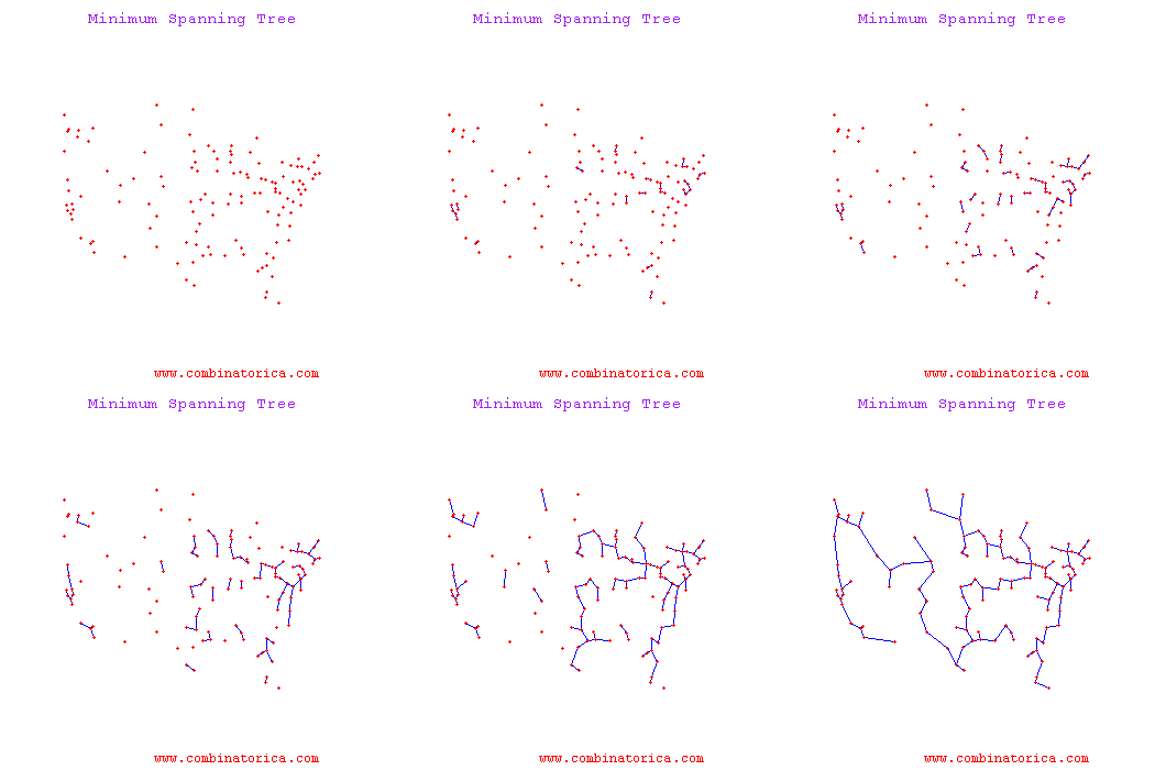
Minimum Spanning Tree Methods (MST)
One can find MST using Prim's Algorithm_OldKiwi (fast test '57) or Krusal's Algorithm_OldKiwi
Kruskal's Algorithm
The algorithm starts with an initial empty tree, and it adds the edge with minimal cost to the tree at each step unless the edge creates a cycle. By repeating this process, it finds a Minimum Spanning tree.
Prim's's Algorithm
Prim's algorithm uses a connected tree as opposed to Kruskal's algorithm. Kruskal's Algorithm searches for minimum cost edge among all edges. Prim's Algorithm starts with the minimum cost edge, then it greedily searches for minimum cost edges among only adjacent edges. When every node is included in the tree algorithm stops.
Zahn's clustering algorithm (1971)
- Find MST
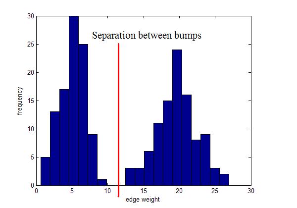
- Identify "inconsistent" edges in MST and remove them.
e.g. remove the longest edge
- edge removed=> 2 clusters
- edges removed=> 3 clusters
What if you have?
Instead, use local inconsistency remove edges significantly larger than their neighborhood edges.
Use for visualization
Visualizations of hierarchical clustering
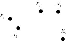
Consider the following set of five 2D data points, which we seek to cluster hierarchically.
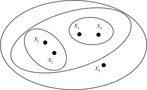
We may represent the hierarchical clustering in various ways. One is by a Venn diagram, in which we circle the data points which belong to a cluster, then subsequently circle any clusters that belong to a larger cluster in the hierarchy.
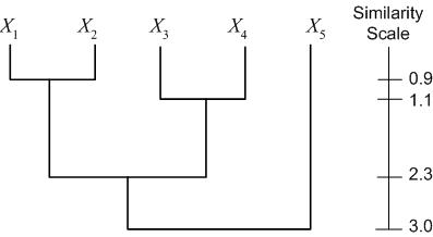
Another representation is a dendogram. A dendogram represents the clustering as a tree, with clusters that are more closely grouped indicated as siblings "earlier" in the tree. The dendogram also includes a "similarity scale," which indicates the distance between the data points (clusters) which were grouped to form a larger cluster. For the example dataset above (with distances calculated as Euclidian distance), we have the following dendogram:
A third representation of hierarchical clustering is by using brackets. We bracket data points/clusters which are grouped into a cluster in a hierarchical fashion as follows: $ \{\{\{X_1,X_2\},\{X_3,X_4\}\},X_5\} $
Agglomerate Algorithms for Hierarchical Clustering (from Distances)
Reference - Chapter 3.2 from Jain and Dudes ??
Begin with a matrix of pairwise distances:
$ \mathcal{D} = \begin{pmatrix} 0 & d_{1,2} & \cdots & d_{1,d} \\ d_{1,2} & 0 & \ddots & \vdots \\ \vdots & \ddots & \ddots & d_{d-1,d} \\ d_{1,d} & \cdots & d_{d-1,d} & 0 \end{pmatrix} $. For simplicity, assume that the distances are pairwise distinct, and sort distances in increasing order: $ d_1, d_2, \cdots, d_{d/2} $
- Begin with clusters $ S_1=\{X_1\}, S_2=\{X_2\}, \cdots, S_d=\{X_d\} $
- Find the two nearest clusters $ S_{i_0}, S_{j_0} $ and merge them into a single cluster
- Repeat step 2 until the number of clusters reaches a pre-specified number (the number 1 corresponds to a dendogram)
Defining Distances Between Clusters
Option 1
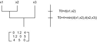
$ {dist}(S_i, S_j) = \min_{X \epsilon S_i, X' \epsilon S_j}{dist}(X, X') $
We call this Nearest Neighbor Distance (NOT a distance, since $ {dist}(S_i, S_j)=0 \not{=>} S_i=S_j $)
This distance choice implies a "Nearest Neighbor (NN) clustering algorithm." Note: At each level of clustering, we have a "single-link clustering" with threshold $ t_0= $ distance between the last two clusters that were merged.
Note: If we continue until all $ X_i $'s are linked, we get MST
Option 2
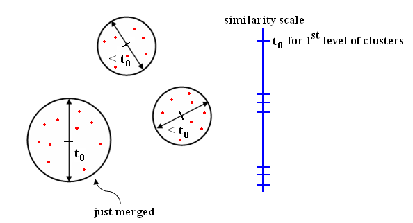
$ {dist}(S_i, S_j) = \max_{X \epsilon S_i, X' \epsilon S_j}{dist}(X, X') $
We call this Farthest Neighbor (FN) Distance.
The Farthest Neighbor Algorithm is also known as The complete linkage clustering. The algorithm tries to estimate "How far the clusters are to each other". In order to find the distance between two clusters, It computes the distance between two farthest points (one from each cluster).
Effect: Increase cluster diameters as little as possible.
- At each level of clustering, you get a complete clustering.
Interpretation of NN and FN algorithm (Johnson-King 1967)
- Input proximity matrix $ \mathcal{D}=(d_{i,j}) $
- Decide which cluster distance you will use (NN, FN, ...)
- Set scale = 0
- Begin with $ S_1=\{X_1\},S_2=\{X_2\},\cdots,S_d=\{X_d\} $
- (*) Find $ (S_{i_0},S_{j_0})=\underset{i \not{=} j}{argmin}({dist}(S_i,S_j)) $ from $ \mathcal{D} $
- Merge $ S_{i_0} $ & $ S_{j_0} $
- Update $ \mathcal{D} $ by deleting rows and columns $ i_0 $ and $ j_0 $; add a row and column for $ S_{d+1}=S_{i_0} \cup S_{j_0} $. Fill in new row and column with the chosen cluster distribution.
- If all objects belong to one single cluster, then stop. Else, goto (*).
Generalization (Lance-William 1967)
Update similarity matrix using formula $ {dist}(S_{i_0} \cup S_{j_0}, S_k) = \alpha_{i_0} d(S_{i_0},S_k)+\beta_{j_0} d(S_{j_0},S_k) + \gamma d(S_{i_0},S_{j_0}) + \delta |d(S_{i_0},S_k)-d(S_{j_0},S_k)| $
Related Websites
- Definition
- Kruskal's algorithm
- Prim's algorithm
- Greedy method
- Definition
- Kruskal's algorithm
- Prim's algorithm
Greedy and Minimum Spanning Algorithms
- Greedy algorithm
- Minimum spanning algorithm
- Kruskal's algorithm
Minmum Spanning Tress(Lecture Note)
- Definition
- Prim-Jarnik's algorithm and example
- Kurskal's algorithm and example
- Baruvka's algorithm and example
Previous: Lecture 23 Next: Lecture 25

