Lecture 8 Lecture notes

Jump to: Outline| 1| 2| 3| 4| 5| 6| 7| 8| 9| 10| 11| 12| 13| 14| 15| 16| 17| 18| 19| 20| 21| 22| 23| 24| 25| 26| 27| 28

Lecture Objective

• Maximum Likelihood Estimation and Bayesian Parameter Estimation
• Linear Discriminant Functions

Maximum Likelihood Estimation and Bayesian Parameter Estimation

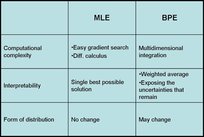
If the prior distributions have some specific properties then the Bayesian Parameter Estimation and Maximum Likelihood Estimation are asymptotically equivalent for infinite training data. However, large training datasets are typically unavailable in pattern recognition problems. Furthermore, when the dimension of data increases, the complexity of estimating the parameters increases exponentially. In that aspect, BPE and MLE have some advantages over each other.

• Computational Complexity:

MLE has a better performance than BPE for large data, because MLE simply uses gradient or differential calculus to estimate the parameters. On the other hand, BPE uses high dimensional integration and it's computationally expensive.

• Interpretability:

The results of MLE are easier to interpret because it generates a single model to fit the data as much as possible. However, BPE generates a weighted sum of models which is harder to understand.

• Form of Distribution:

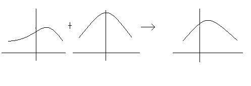
The advantage of using BPE is that it uses prior information that we have about the model and it gives us a possibility to sequentially update the model. If the information we have on the model is reliable than BPE is better than MLE. On the other hand, if prior model is uniformly distributed than BPE is not so different than MLE. Indeed, MLE is a special and simplistic form of BPE.

Figure for BPE processes:

See also: Comparison of MLE and Bayesian Parameter Estimation

Linear Discriminant Functions

(From DHS Chapter 5)

Suppose we have $ p(w_1|\vec{x}) $ and $ p(w_2|\vec{x}) $

$ g(\vec{x}) = p(w_1|\vec{x}) - p(w_2|\vec{x}) $

$ p(\vec{x}|w_i) $ -> Parametric Estimation Method

$ g(\vec{x}) $ -> proper form of Linear Discriminant Function

$ [1,x,x^2,x^3] $ -> new feature space

Simple and easy to design:

• 1 category case:

$ g(\vec{x}) = w\vec{x} + w_0 $

where $ w $ is the weight factor and $ w_0 $ is the bias of the threshold

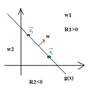
• 2 category case:

$ w_1, g(\vec{x}) > 0 $

$ w_2, g(\vec{x}) < 0 $

$ g(\vec{x}) = 0 $ : decision surface

$ g(\vec{x_1}) = w'\vec{x_1} + w_0 $

$ g(\vec{x_2}) = w'\vec{x_2} + w_0 $

$ w'\vec{x_1} + w_0 = w'\vec{x_2} + w_0 $

$ w'(\vec{x_1} - \vec{x_2}) = 0 $

• N category case:

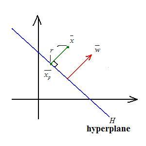
$ \vec{x} = \vec{x_p} + r\frac{\vec{w}}{|\vec{w}|} $

where $ \vec{x_p} $ is the projection point, $ r $ is the distance, and $ \frac{\vec{w}}{|\vec{w}|} $ is the unit normal

$ g(\vec{x}) = w'\vec{x} + w_0 = w'(\vec{x_p} + r\frac{\vec{w}}{|\vec{w}|}) + w_0 = w'\vec{x_p} + w_0 + w'r\frac{\vec{w}}{|\vec{w}|} = r|\vec{w}| $

therefore $ r = \frac{g(\vec{x})}{|\vec{w}|} $

For more information:

Parametric Estimators

Previous: Lecture 7 Next: Lecture 9

Back to ECE662 Spring 2008 Prof. Boutin