Lecture 27 Lecture notes

Jump to: Outline| 1| 2| 3| 4| 5| 6| 7| 8| 9| 10| 11| 12| 13| 14| 15| 16| 17| 18| 19| 20| 21| 22| 23| 24| 25| 26| 27| 28

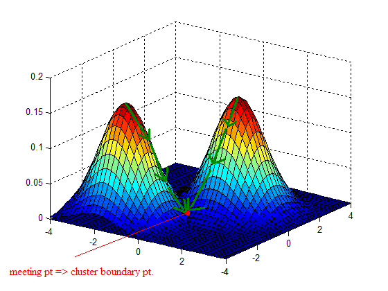
Clustering by finding valleys of densities

-- Approach 1: "Bump Hunting" --

   - Approximate p(x)
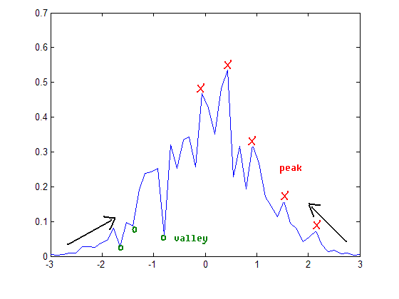
   - Find peaks of density
   - Expand cluster boundaries outward until they meet (hopefully in middle!)
   - Define meeting points = Cluster boundary points

(fig.1)

-- Approach 2: "Valley Seeking" --

   - Start from valley regions of p(x)
   - Work uphill to connect data points to density peaks

(fig.2)

Graph based implementation

   - Estimate p(x)
   - For all patterns $ X_i $, denote by $ N_r(X_i) $, the neighborhood of size $ r $ of $ X_i $.
   - Estimate derivative of density p(x) along direction $ X_i-X_j, \forall X_j\in N_r(X_i) $
           $ S_i(j)=\frac{p(X_i)-p(X_j)}{||X_i-X_j||_{L_2}} $
           Let $ j_{max}=argmax_j S_i(j) $
           If $ S_i(j_{max})<0 $ declare $ i $ to be a root node.
           If $ S_i(j_{max})>0 $ declare $ X_{j_{max}} $ to be parent of $ X_i $.
           If $ S_i(j_{max})=0 $ it depends on the surroundings what link we establish.
   - If $ X_i $ is connected to a root node, then make this root node a parent of $ X_i $, else make $ X_i $ a root node.
   - Repeat

When all points are visited, a forest is constructed. Each connected component (=tree of a forest) is a cluster.

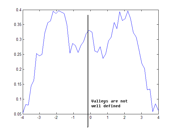
• Problem: All methods presented above encounter a serious problem because of the following reasons:

   - Density may oscillate a lot
   - Valleys are not well defined.

(fig.3)

PDE based valley seeking

PDE: Partial Differential Equation

PDE's can be used to minimize energy functionals

• Simple Example

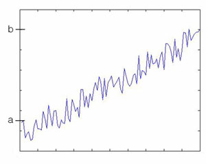
Consider 1-D curves

$ u(x): [0,1] \rightarrow \Re $ with fixed end points $ u(0)=a $, $ u(1)=b $ (3-1)

Suppose Energy of curve is $ E(u)=\int _0 ^1 F(u, u')dx $ for some function $ F: \Re ^2 \rightarrow \Re $

e.g.) $ F(u,u')=|u'|^2 $ (3-2)

The curve that minimizes (or maximizes) E(u) satisfies Euler Equation

$ \frac{\partial F} {\partial u} -\frac{d}{dx}(\frac{\partial F}{\partial u'})=0 $ (3-3)

sometimes written as $ E'=0 \Rightarrow \frac{\partial E}{\partial u}=0 $ (3-4)

Similarly if $ E=\int _0 ^1 F(u,u',u'')dx $ (3-5)

e.g.) $ F(u,u',u'')=|u''|^2 $ (3-6)

Then Euler equation is $ \frac{\partial F}{\partial u} - \frac{d}{dx}(\frac{\partial F}{\partial u'}) + \frac{d^2}{dx^2}(\frac{\partial F}{\partial u''})=0 $ (3-7)

Similarly, for surface in $ \Re ^2 $

$ u(x,y): [0,1] \times [0,1] \rightarrow \Re $ (3-8)

Suppose energy is given by

$ E(u)=\int _{surface} F(u,u_x, u_y, u_{xx}, u_{xy},u_{yy})dxdy $ (3-9)

e.g.) $ F={u_x}^2+{u_y}^2 $ (3-10)

Then Euler equation is

$ \frac{\partial F}{\partial u} - \frac{d}{dx}(\frac{\partial F}{\partial u_x}) - \frac{d}{dy}(\frac{\partial F}{\partial u_y}) + \frac{d^2}{dx^2}(\frac{\partial F}{\partial u_{xx}}) + \frac{d^2}{dy^2}(\frac{\partial F}{\partial u_{yy}}) + \frac{d^2}{dxdy}(\frac{\partial F}{\partial u_{xy}})=0 $ (3-11)

• Illustration

1D curve $ u(x) $ with $ u(0)=a, u(1)=b $ (3-12)

$ E(u)=\int _{0} ^{1} ||\nabla u||^2 dx $ (3-13) Dirichlet integral

$ F=||\nabla u||^2=u_x ^2 $

Euler equation E'=0

$ \frac{\partial F}{\partial u} - \frac{d}{dx}(\frac{\partial F}{\partial u_x})=0 $ (3-14)

$ 0-\frac{d}{dx}(2u_x)=0 \Rightarrow -2u_{xx}=0 \Rightarrow u_{xx}=0 $ (3-15)

with boundary condition, $ u(0)=0, u(1)=b $

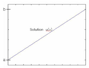
Solution: $ u(x)=c_1 x+ c_2 $

$ u(0)=a \Rightarrow c_2=a $ (3-16)

$ u(1)=b \Rightarrow c_1 + c_2 = b \Rightarrow c_1=b-a $ (3-17)

In general, cannot solve Euler equation analytically

In practice, use 'Gradient descent'

Pick initial curve $ u_0 (x) $

Consider a family of curves $ u(t,x) $ such that $ u(0,x)=u_0 (x) $ and $ \frac{\partial u}{\partial t}= \pm E' $ (3-18)

+: if looking for max

-: if looking for min

t is called "time marching parameter"

Solve for $ u(t,x) $ numerically, when "steady state" $ \frac{\partial u}{\partial E}=0 $ is achieved. (3-19)

Say at $ u(t_{final},x)=: u_1 (x) $ (3-20)

Then $ u_1(x) $ is the solution to Euler Equation $ E'=0 $

• Example

$ F=||\nabla u||^2 = u_x ^2 $ (3-21)

Look for curve $ u(x) $ such that $ u(0)=a, u(1)=b $ with minimum E. (3-22)

Consider $ u(t,x) $

$ u(0,x) $ is initial guess

Gradient descent (Equation to Euler's equation)

$ \frac{\partial u}{\partial t}=u_{xx} $ "Heat Equation" (3-23)

<<Picture>>

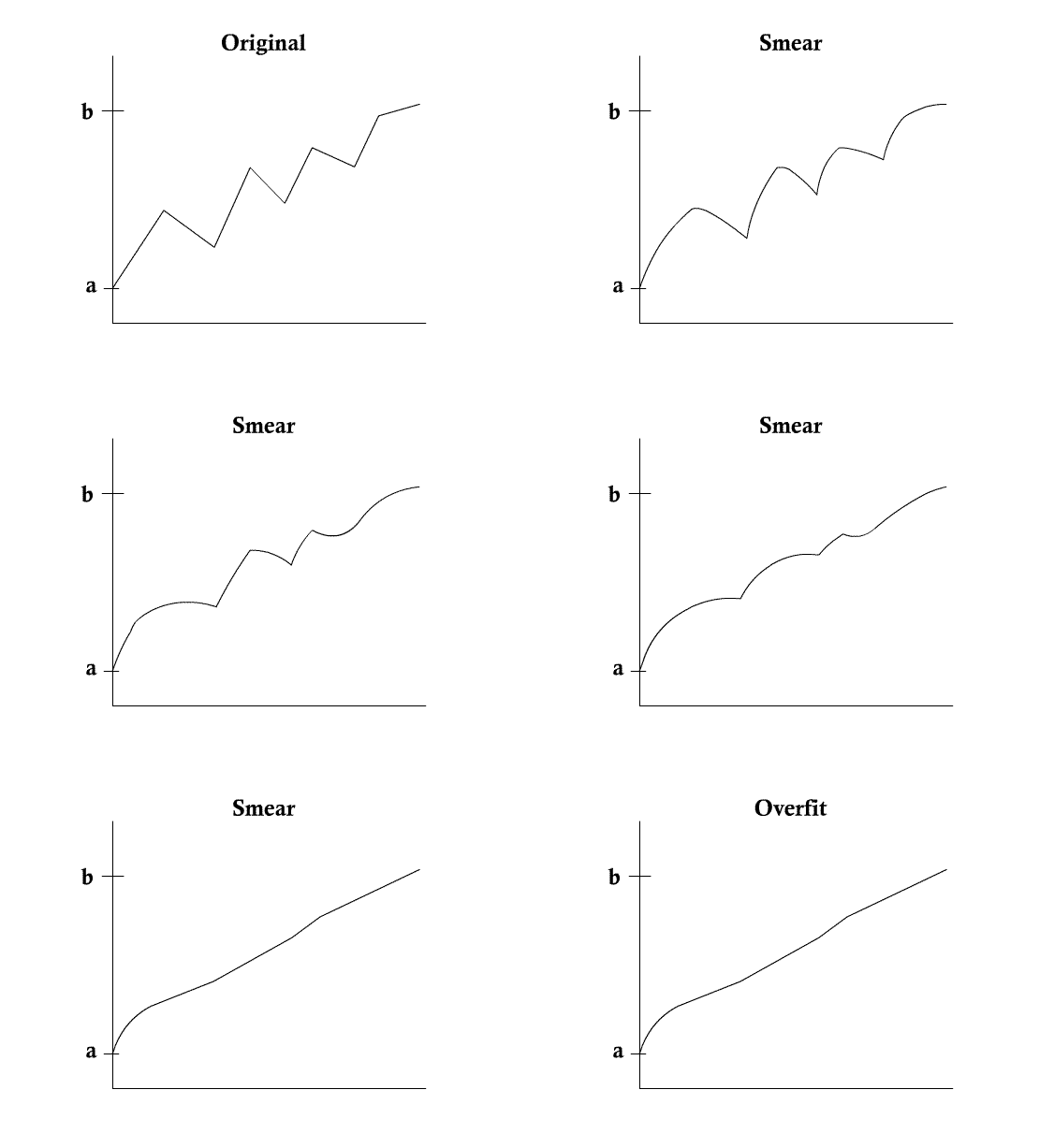
• curve gets less and less curvy as t evolves
• in fact, evolving for t units is equivalent to convolving $ u_0 (x) $ with Gaussian kernel

$ G(x,t)=\sqrt{\frac{1}{4 \pi t}} e^{-\frac{x^2}{4t}} $ (3-24)

i.e., $ u(t,x)=u_0 (x) * G(x,t) $

<<Figure>>

Scale space of curves

If cannot solve $ \frac{\partial u}{\partial t}=E' $ discretize and solve numerically (3-25)

$ \frac{\partial u}{\partial t} \approx \frac{u(t+ \Delta t ,x )-u(t,x)}{\Delta t} $ (3-26)

$ u_{xx} \approx \frac{u(t,x+\Delta x)-2u(t,x)+u(t,x-\Delta x)}{\Delta x^2} $ (3-27)

$ \frac{\partial u}{\partial t}=u_{xx} $ (3-28)

$ \frac{u(t+\Delta t,x)-u(t,x)}{\Delta t}=\frac{u(t,x+\Delta x)-2u(t,x)+u(t,x-\Delta x)}{\Delta x^2} $ (3-29)

$ u(t+\Delta t, x)=u(t,x)+\frac{\Delta t}{\Delta x^2}(u(t,x+\Delta x)-2u(t,x)+u(t,x-\Delta x)) $ (3-30)