Lecture 11 Lecture notes

Jump to: Outline| 1| 2| 3| 4| 5| 6| 7| 8| 9| 10| 11| 12| 13| 14| 15| 16| 17| 18| 19| 20| 21| 22| 23| 24| 25| 26| 27| 28

Derivation of Fischer's Linear Discriminant

Main article: Derivation of Fisher's Linear Discriminant

The derivation was completed in this lecture.

Recall from last lecture

Last time, we considered

$ J(\vec{w}) = \frac{\vec{w}^t S_B \vec{w}}{\vec{w}^t S_W \vec{w}} $

which is explicit function of $ \vec{w} $

One can do this because numerator of $ J(\vec{w}) $ can be written as

$ \mid \tilde m_1 - \tilde m_2 \mid^2 = \mid w \cdot (m_1 - m_2) \mid^2 = w^t (m_1 - m_2) (m_1^t - m_2^t) w $

$ \rightarrow S_B = (m_1 - m_2) (m_1^t - m_2^t) $

In a same way, denominator can be written as

$ \tilde s_1^2 + \tilde s_2^2 = \sum_{y_i \in class \ i} (w \cdot y_i - \tilde m_1)^2 = \sum w^t (y_i - m_i)(y_i^t - m_i^t) w $

$ = w^t \left[ \sum (y_i - m_i)(y_i^t - m_i^t) \right] w $

$ \rightarrow S_W = \sum_{y_i \in class \ i} (y_i - m_i)(y_i^t - m_i^t) $

Fisher Linear Discriminant

It is a known result that J is maximum at $ \omega_0 $ such that $ S_B\omega_0=\lambda S_W\omega_0 $. This is the "Generalized eigenvalue problem.

Note that if $ |S_W|\neq 0 $, then $ {S_W}^{-1}S_B\omega_0=\lambda\omega_0 $. It can be written as the "Standard eigenvalue problem". The only difficulty (which is a big difficulty when the feature space dimension is large) is that matrix inversion is very unstable.

Observe that $ S_B\omega_0=(\vec{m_1}-\vec{m_2})(\vec{m_1}-\vec{m_2})^T\omega_0=cst.(\vec{m_1}-\vec{m_2}) $. Therefore the standard eigenvalue problem as presented above becomes $ {S_W}^{-1}cst.(\vec{m_1}-\vec{m_2})=\lambda\omega_0 $. From this equation, value of $ \omega_0 $ can easily be obtained, as $ \omega_0={S_W}^{-1}(\vec{m_1}-\vec{m_2}) $ or any constant multiple of this. Note that magnitude of $ \omega_0 $ is not important, the direction it represents is important.

Fischer's Linear Discriminant in Projected Coordinates

Claim

$ \vec{c}=\omega_0={S_W}^{-1}(\vec{m_1}-\vec{m_2}) $

is the solution to $ \mathbf{Y}\vec{c}=\vec{b} $ with $ \vec{b}=(d/d_1, \cdots, <d_1 times>, d/(d-d_1), \cdots, <(d-d_1) times>)^T $

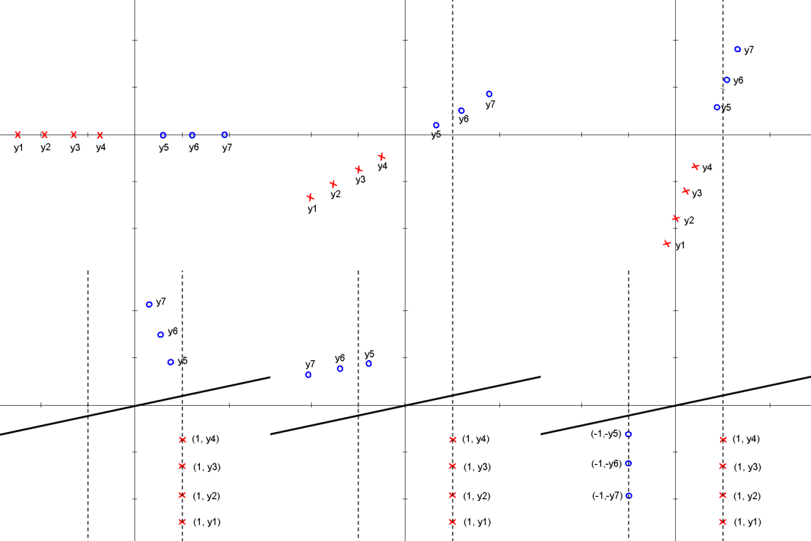
Here is an animation of the 1D example given in class on projections

Explanation

starts with $ \vec{\omega} \cdot y_i + \omega_0 > 0 $ for class 1 and $ \vec{\omega} \cdot y_i + \omega_0 < 0 $ for class 2

the data points are then projected onto an axis at 1 which results in

$ \vec{\omega} \cdot y_i > 0 $ for class 1 and $ \vec{\omega} \cdot y_i < 0 $ for class 2

one class is then projected onto an axis at -1 which results in

$ \vec{\omega} \cdot y_i > 0 $ for all $ y_i $

Support Vector Machines (SVM)

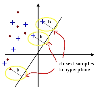
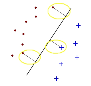
A support vector for a hyperplane $ \vec{c} $ with margin $ b_i \geq b $ is a sample $ y_{io} $ such that $ c\cdot{y_{io}} = b $.

Support Vector Machines are a two step process:

1) Preprocessing - X1,...,Xd features in kth dimensional real space is mapped to features in n dimensional real space where n>>k.

2) Linear Classifier - separates classes in n dimensional real space via hyperplane. - Support Vectors - for finding the hyperplane with the biggest margins. - Kernel - to simplify computation (This is key for real world applications)

Previous: Lecture 10. Next: Lecture 12

Back to ECE662 Spring 2008 Prof. Boutin