Lecture 17 Lecture notes

Jump to: Outline| 1| 2| 3| 4| 5| 6| 7| 8| 9| 10| 11| 12| 13| 14| 15| 16| 17| 18| 19| 20| 21| 22| 23| 24| 25| 26| 27| 28

Nearest Neighbor Classification Rule

• useful when there are several labels
• e.g. fingerprint-based recognition

Problem: Given the labeled training samples: $ \vec{X_1}, \vec{X_2}, \ldots, \vec{X_d} $ $ \in \mathbb{R}^n $ (or some other feature space) and an unlabeled test point $ \vec{X_0} $ $ \in \mathbb{R}^n $.

Classification: Let $ \vec{X_i} $ be the closest training point to $ \vec{X_0} $, then we assign the class of $ \vec{X_i} $ to $ \vec{X_0} $.

What do we mean by closest?

There are many meaning depending on the metric we choose for the feature space.

Definition A "metric" on a space S is a function

$ D: S\times S\rightarrow \mathbb{R} $

that satisfies the following 4 properties:

• Non-negativity $ D(\vec{x_1},\vec{x_2})\geq 0, \forall \vec{x_1},\vec{x_2}\in S $
• Symmetry $ D(\vec{x_1},\vec{x_2})=D(\vec{x_2},\vec{x_1}), \forall \vec{x_1},\vec{x_2}\in S $
• Reflexivity $ D(\vec{x},\vec{x})=0, \forall \vec{x}\in S $
• Triangle Inequality $ D(\vec{x_1},\vec{x_2})+D(\vec{x_2},\vec{x_3})\geq D(\vec{x_1},\vec{x_3}) , \forall \vec{x_1}, \vec{x_2}, \vec{x_3}\in S $

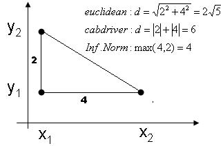
Illustration of 3 different metrics

Examples of metrics

Euclidean distance: $ D(\vec{x_1},\vec{x_2})=||\vec{x_1}-\vec{x_2}||_{L_2}=\sqrt{\sum_{i=1}^n ({x_1}^i-{x_2}^i)^2} $

Manhattan (cab driver) distance: $ D(\vec{x_1},\vec{x_2})=||\vec{x_1}-\vec{x_2}||_{L_1}=\sum_{i=1}^n |{x_1}^i-{x_2}^i| $

Minkowski metric: $ D(\vec{x_1},\vec{x_2})=||\vec{x_1}-\vec{x_2}||_{L_p}=(\sum_{i=1}^n ({x_1}^i-{x_2}^i)^p)^{\frac{1}{p}} $

Riemannian metric: $ D(\vec{x_1},\vec{x_2})=\sqrt{(\vec{x_1}-\vec{x_2})^\top \mathbb{M}(\vec{x_1}-\vec{x_2})} $

Infinite norm: $ D(\vec{x_1},\vec{x_2})=||\vec{x_1}-\vec{x_2}||_{\infty}=max_i |{x_1}^i-{x_2}^i| $

where M is a symmetric positive definite $ n\times n $ matrix. Different choices for M enable associating different weights with different components.

In this way, we see that $ \mathbb{R}^n $, $ \mathbb{Z}^n $, $ \mathbb{C}^n $ have many natural metrics, but feature could be in some other set, e.g. a discrete set.

for example,

$ x_1 $={fever, skinrash, high blodd pressure}

$ x_2 $={fever, neckstiffness}

Tanimoto metric

$ D(set1, set2) = \frac {|set1|+|set2|-2|set1 \bigcap set2| }{|set1|+|set2|-|set1 \bigcap set2|} $

Example: previous approach to shape recognition Given is a set of ordered points in $ R_n =(p_1,p_2,\cdots,p_N) $ We want to recognize the shape

Figure 1

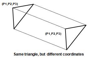
Given template (triangle form): (T1,T2,...,TN); We want to assign one of test template to a test (P1,P2,P3) In this case, we should not use Euclidean distance!,

Figure 2

becasue shape defined by point is unchanged (invariant) by rotation and translation of triangles.

Therefore, distance between 2 triangles (or shapes) must be independent on the position and orientation of triangles.

Procrustes metric

$ D(p,\bar p)= \sum_{\begin{matrix}i=1 \\ rotation R, translation T \end{matrix}}^n {\begin{Vmatrix} Rp_i+T-\bar p_i \end{Vmatrix}} _{L^2} $

$ p=(p_1, p_2, \cdots ,p_N),\bar p = (\bar p_1, \bar p_2, \cdots ,\bar p_N) $

Alternative approach "Use invariant coordinate to repeat $ p=(p_1, p_2, \cdots ,p_N) $ "

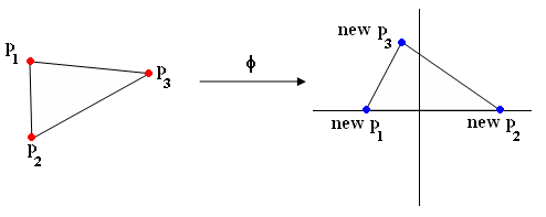
i.e find $ \varphi $ such that

$ \varphi : \mathbb{R}^n\rightarrow \mathbb{R}^k $ (where, typically $ k \leq n $)

s.t $ \varphi (x) = \varphi (\bar x) $

whenever $ \exists $ R, T with $ R \bar X + \bar T = X $

Example of phi with triangle (Figure 3):

(p1,p2,p3) -> (new p1, new p2, new p3)

Previous: Lecture 16 NextLecture 18

Back to ECE662 Spring 2008 Prof. Boutin