Lecture 13 Lecture notes

Jump to: Outline| 1| 2| 3| 4| 5| 6| 7| 8| 9| 10| 11| 12| 13| 14| 15| 16| 17| 18| 19| 20| 21| 22| 23| 24| 25| 26| 27| 28

(continued from Lecture 12)

Kernel Functions

Kernel Functions

Last class introduced kernel functions trick as a key to make SVM an effective tool for classifying linearly separable data. Here we see some examples of kernel functions, and the condition that determined if these functions correspond to dot product in some feature space.

Note that $ \varphi $can be a mapping as $ \varphi:\Re^k\rightarrow\mathbb{H} $

where $ \mathbb{H} $ can be $ \infty $ dimensional.

Here is the example of a "Gaussian Kernel" with $ \varphi $ as $ \infty $ dimensional. $ k(\vec{x},\vec{x'})=e^{-\frac{||\vec{x}-\vec{x}||^2}{2\sigma^2}} $, $ \sigma $ parameter.

It is easier to work with $ k(\vec{x},\vec{x'}) $ than with $ \varphi(\vec{x}) $.

In this example, computation of the dot product $ \varphi(\vec{x}) \cdot \varphi(\vec{x'}) $requires infinite summation. Kernel function allows us to compute distance to hyperplane with same computational cost as training SVM in initial data space.

For which kernel does there exist a mapping to a higher dimensional space?

The answer lies in Mercer's Condition (Covrant and Hilbert in '53; Vapnik in '95)

Given a kernel $ K:\Re ^k \times \Re ^k \rightarrow \Re $, there exists a $ \varphi $ and an expansion

$ k(\vec{x},\vec{x'})=\sum_{i}\varphi(\vec{x})_{i}\varphi(\vec{x'})_{i} $, where i could range in infinite space

$ \Longleftrightarrow \forall g(\vec{x}) $ $ \int [g(\vec{x})]^{2}d\vec{x}<\infty $

$ \int\int k(\vec{x},\vec{x'})g(\vec{x})g(\vec{x'})d\vec{x}d\vec{x'}\geq 0 $

This condition is satisfied for $ k(\vec{x},\vec{x'})=||\vec{x}-\vec{x'}||^p $ for any $ p\in \mathbb{N} $

In this case, $ \varphi $ is a polynomial mapping, homogeneous with degree p in each component.

e.g. $ \varphi(\vec{x})=(\varphi_{r_1r_2\ldots r_{d_L}}(\vec{x})) $ where $ \varphi_{r_1r_2\ldots r_{d_L}}(\vec{x})=(\sqrt{\frac{p!}{r_{1}!\ldots r_{d_L}!}}){x_1}^{r_1}\ldots {x_{d_L}}^{r_{d_L}} $

and

$ \sum_{i=1}^{d_L}r_i=p $, $ r_i\geq 0 $

Example : $ p(x,y)=7x^2-14y^2+3xy $

To visualize the separation surface we need to find x and y such that:

$ p(x,y)=0 $

To solve such equation, we could take a segment of y and divide it on intervals. On each interval we fix a value of y and solve the quadratic function for x. Then, we connect the resulting points to see the surface. This example is illustrated on the figure below this paragraph.

.. image:: mortiz_lec13.gif

align: center

Artificial Neural Networks

What is a Neural Network?

An [Artificial Neural Network] is an information processing paradigm that is inspired by the way biological nervous systems, such as the brain, process information. The key element of this paradigm is the novel structure of the information processing system. It is composed of a large number of highly interconnected processing elements (neurones) working in unison to solve specific problems. ANNs, like people, learn by example. An ANN is configured for a specific application, such as pattern recognition or data classification, through a learning process. Learning in biological systems involves adjustments to the synaptic connections that exist between the neurones. This is true of ANNs as well.

General Properties:

Neural networks, with their remarkable ability to derive meaning from complicated or imprecise data, can be used to extract patterns and detect trends that are too complex to be noticed by either humans or other computer techniques. A trained neural network can be thought of as an "expert" in the category of information it has been given to analyze. This expert can then be used to provide projections given new situations of interest and answer "what if" questions. Other advantages include:

1. Adaptive learning: An ability to learn how to do tasks based on the data given for training or initial experience. 2. Self-Organization: An ANN can create its own organization or representation of the information it receives during learning time.

Neural networks are a family of function approximation techniques, when the function is approximated,

$ f:x \rightarrow z $ (1)

is modeled as a composition of simple functions $ f_i's $

$ f=f_n\bullet f_{n-1}\cdot\cdot\cdot f_1 $ (2)

The composition model is represented by a network

Several $ f_i's $ are taken to be linear functions

The parameters of the linear functions are optimized to best fit the data

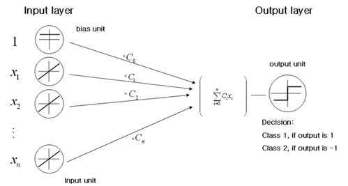
Example) [Linear Discriminant Functions] can be seen as a two layer Neural Network(NN)

recall $ g(\vec{x})=\vec{c}\cdot (1,\vec{x}) $ (3)

$ g(\vec{x}) > 0 \Rightarrow class 1 , < 0 \Rightarrow class 2 $ (4)

write

$ \vec{x} = \begin{pmatrix} x_1 \\ x_2 \\ x_3 \\ \vdots \\ x_n \end{pmatrix} $ (5)

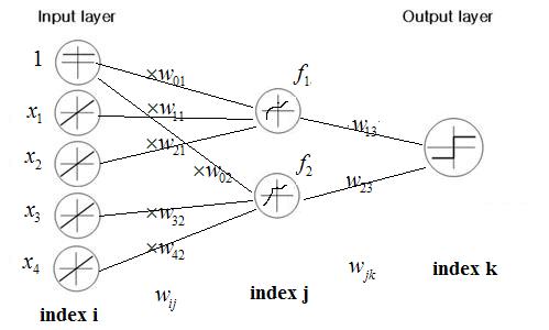
Example of three layer NN

Common types of function fi's

linear: $ f(\vec x)=\vec c^T\vec x+c_0 $ (6)

logistic: $ f(x)=\frac{e^x}{1+e^x} $ (7)

threshold: $ f(x)=1,x>0;f(x)=0,else $ (8)

hyperbolic tangent: $ f(x)=\frac{e^x-1}{e^x+1} $ (9)

sign function: $ f(x)=1,x>0;f(x)=-1,else $ (10)

any continuous $ g(\vec x):[0,1]*[0,1]*...*[0,1]\rightarrow\Re $ (11)

can be written as :

$ g(\vec{x})=\sum _{j=1}^{2n+1} G_j(\sum _{i} \psi _{ij} (x_i)) $ (12)

Training Neural Networks - "Back-Propagation Algorithm"

First define a cost function to measure the error of the neural network with weights $ \vec{w} $, say we have training input values $ \vec{x_k} $ => output $ z_k $, but desire output $ t_k $.

This cost function can be written as below

$ J(\vec{w}) = \frac{1}{2} \sum_{k} (t_k - z_k)^2 = \frac{1}{2} \mid \vec{t} - \vec{k} \mid ^2 $ (13)

Then, we can optimize this cost function using gradient descent method

new $ \vec{w}= $ old $ \vec{w}+ \Delta \vec{w} $ (14)

$ \rightarrow \vec{w}(k+1) = \vec{w}(k) - \eta(k) \left( \frac{\partial J}{\partial w_1}, \frac{\partial J}{\partial w_2}, \cdots , \frac{\partial J}{\partial w_{last}} \right) $ (15)

Previous: Lecture 12 Next: Lecture 14

Back to ECE662 Spring 2008 Prof. Boutin