ECE662: Statistical Pattern Recognition and Decision Making Processes
Spring 2008, Prof. Boutin
Collectively created by the students in the class
Contents
[hide]Lecture 7 Lecture notes
Jump to: Outline| 1| 2| 3| 4| 5| 6| 7| 8| 9| 10| 11| 12| 13| 14| 15| 16| 17| 18| 19| 20| 21| 22| 23| 24| 25| 26| 27| 28
Lecture Content
- Maximum Likelihood Estimation and Bayesian Parameter Estimation
- Parametric Estimation of Class Conditional Density
Relevant Links
- MLE:
- BPE:
- More on Parametric Extimators
The class conditional density $ p(\vec{x}|w_i) $ can be estimated using training data. We denote the parameter of estimation as $ \vec{\theta} $. There are two methods of estimation discussed.
MLE Maximum Likelihood Estimation
BPE Bayesian Parameter Estimation
Maximum Likelihood Estimation
Let "c" denote the number of classes. D, the entire collection of sample data. $ D_1, \ldots, D_c $ represent the classification of data into classes $ \omega_1, \ldots, \omega_c $. It is assumed that: - Samples in $ D_i $ give no information about the samples in $ D_j, i \neq j $, and - Each sample is drawn independently.
Example: The class conditional density $ p(\vec{x}|w_i) $ depends on parameter $ \vec{\theta_i} $. If $ X ~ N(\mu,\sigma^2) $ denotes the class conditional density; then $ \vec{\theta}=[\mu,\sigma^2] $.
Let n be the size of training sample, and $ D=\{\vec{X_1}, \ldots, \vec{X_n}\} $. Then,
$ p(\vec{X}|\omega_i,\vec{\theta_i}) $ equals $ p(\vec{X}|\vec{\theta}) $ for a single class.
The Likelihood Function is, then, defined as $ p(D|\vec{\theta})=\displaystyle \prod_{k=1}^n p(\vec{X_k}|\vec{\theta}) $, which needs to be maximized for obtaining the parameter.
Since logarithm is a monotonic function, maximizing the Likelihood is same as maximizing log of Likelihood which is defined as
$ l(\vec{\theta})=log p(D|\vec{\theta})=\displaystyle log(\prod_{k=1}^n p(\vec{X_k}|\vec{\theta}))=\displaystyle \sum_{k=1}^n log(p(\vec{X_k}|\vec{\theta})) $.
"l" is the log likelihood function.
Maximize log likelyhood function with respect to $ \vec{\theta} $
$ \rightarrow \hat{\theta} = argmax \left( l (\vec{\theta}) \right) $
If $ l(\vec{\theta}) $ is a differentiable function
Let $ \vec{\theta} = \left[ \theta_1, \theta_2, \cdots , \theta_p \right] $ be 1 by p vector, then
$ \nabla_{\vec{\theta}} = \left[ \frac{\partial}{\partial\theta_1} \frac{\partial}{\partial\theta_2} \cdots \frac{\partial}{\partial\theta_p} \right]^{t} $
Then, we can compute the first derivatives of log likelyhood function,
$ \rightarrow \nabla_{\vec{\theta}} ( l (\vec{\theta}) ) = \sum_{k=1}^{n} \nabla_{\vec{\theta}} \left[ log(p(\vec{x_k} | \vec{\theta})) \right] $
and equate this first derivative to be zero
$ \rightarrow \nabla_{\vec{\theta}} ( l (\vec{\theta}) ) = 0 $
Example of Guassian case
Assume that covariance matrix are known.
$ p(\vec{x_k} | \vec{\mu}) = \frac{1}{ \left( (2\pi)^{d} |\Sigma| \right)^{\frac{1}{2}}} exp \left[ - \frac{1}{2} (\vec{x_k} - \vec{\mu})^{t} \Sigma^{-1} (\vec{x_k} - \vec{\mu}) \right] $
Step 1: Take log
$ log p(\vec{x_k} | \vec{\mu}) = -\frac{1}{2} log \left( (2\pi)^d |\Sigma| \right) - \frac{1}{2} (\vec{x_k} - \vec{\mu})^{t} \Sigma^{-1} (\vec{x_k} - \vec{\mu}) $
Step 2: Take derivative
$ \frac{\partial}{\partial\vec{\mu}} \left( log p(\vec{x_k} | \vec{\mu}) \right) = \frac{1}{2} \left[ (\vec{x_k} - \vec{\mu})^t \Sigma^{-1}\right]^t + \frac{1}{2} \left[ \Sigma^{-1} (\vec{x_k} - \vec{\mu}) \right] = \Sigma^{-1} (\vec{x_k} - \vec{\mu}) $
Step 3: Equate to 0
$ \sum_{k=1}^{n} \Sigma^{-1} (\vec{x_k} - \vec{\mu}) = 0 $
$ \rightarrow \Sigma^{-1} \sum_{k=1}^{n} (\vec{x_k} - \vec{\mu}) = 0 $
$ \rightarrow \Sigma^{-1} \left[ \sum_{k=1}^{n} \vec{x_k} - n \vec{\mu}\right] = 0 $
$ \Longrightarrow \hat{\vec{\mu}} = \frac{1}{n} \sum_{k=1}^{n} \vec{x_k} $
This is the sample mean for a sample size n.
MLE Examples: Exponential and Geometric Distributions
[MLE Examples: Binomial and Poisson Distributions
Advantages of MLE:
- Simple
- Converges
- Asymptotically unbiased (though biased for small N)
Bayesian Parameter Estimation
For a given class, let $ x $ be feature vector of the class and $ \theta $ be parameter of pdf of $ x $ to be estimated.
And let $ D= \{ x_1, x_2, \cdots, x_n \} $ , where $ x $ are training samples of the class
Note that $ \theta $ is random variable with probability density $ p(\theta) $
where
Here is a good example .
EXAMPLE: Bayesian Inference for Gaussian Mean
The univariate case. The variance is assumed to be known.
Here's a summary of results:
- Univariate Gaussian density $ p(x|\mu)\sim N(\mu,\sigma^{2}) $
- Prior density of the mean $ p(\mu)\sim N(\mu_{0},\sigma_{0}^{2}) $
- Posterior density of the mean $ p(\mu|D)\sim N(\mu_{n},\sigma_{n}^{2}) $
where
- $ \mu_{n}=\left(\frac{n\sigma_{0}^{2}}{n\sigma_{0}^{2}+\sigma^{2}}\right)\hat{\mu}_{n}+\frac{\sigma^{2}}{n\sigma_{0}^{2}+\sigma^{2}}\mu_{0} $
- $ \sigma_{n}^{2}=\frac{\sigma_{0}^{2}\sigma^{2}}{n\sigma_{0}^{2}+\sigma^{2}} $
- $ \hat{\mu}_{n}=\frac{1}{n}\sum_{k=1}^{n}x_{k} $
Finally, the class conditional density is given by $ p(x|D)\sim N(\mu_{n},\sigma^{2}+\sigma_{n}^{2}) $
The above formulas can be interpreted as: in making prediction for a single new observation, the variance of the estimate will have two components: 1) $ \sigma^{2} $ - the inherent variance within the distribution of x, i.e. the variance that would never be eliminated even with perfect information about the underlying distribution model; 2) $ \sigma_{n}^{2} $ - the variance introduced from the estimation of the mean vector "mu", this component can be eliminated given exact prior information or very large training set ( N goes to infinity);

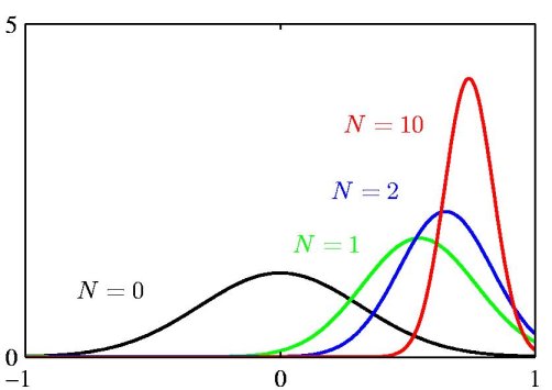
The above figure illustrates the Bayesian inference for the mean of a Gaussian distribution, for which the variance is assumed to be known. The curves show the prior distribution over 'mu' (the curve labeled N=0), which in this case is itself Gaussian, along with the posterior distributions for increasing number N of data points. The figure makes clear that as the number of data points increase, the posterior distribution peaks around the true value of the mean. This phenomenon is known as *Bayesian learning*.
For more information:


