ECE662: Statistical Pattern Recognition and Decision Making Processes

Spring 2008, Prof. Boutin

sLecture

Collectively created by the students in the class

---

Lecture 26 Lecture notes

Quick link to lecture notes: 1| 2| 3| 4| 5| 6| 7| 8 9| 10 11| 12| 13| 14| 15| 16| 17| 18| 19| 20| 21| 22| 23| 24| 25| 26| 27| 28

---

---

Assignment Update

• There will not be a final project homework assignment, instead a peer review of the last homework will take place see Homework 3_OldKiwi for details.

Clustering

• There are no best criterion for obtaining a partition of $ \mathbb{D} $
• Each criterion imposes a certain structure on the data.
• If the data conforms to this structure, the true clusters can be discovered.
• There are very few criteria which can be both handled mathematically and understood intuitively. If you can develope a useful intuitive criterion and describe and optimize it mathematically, you can make big contributions to this field.
• Some criteria can be written in different ways, for example minimizing the square error, as in the following section.

Minimizing

$ J=\sum_{j=1}^c\sum_{x_{i}\in S_{j}}||x_{i}-\mu_{j}||^{2} $ $ =\sum_{j=1}^c\frac{1}{|S_{j}|}\sum_{x_{i},x_{k}\in S_{j}}||x_{i}-x_{k}||^{2}is $

same as minimizing trace of the within class variation matrix,

$ J_{within}=\sum_{j=1}^c\sum_{x_{i}\in S_{j}}(x_{i}-\mu_{j})^{T}(x_{i}-x_{j})=\sum_{j=1}^c\sum_{x_{i}\in S_{j}}tr((x_{i}-\mu_{j})(x_{i}-x_{j})^{T}) $ which is the same as maximizing the between-cluster variance$ S_{Total}=S_{W}+S_{B} $ $ tr(S_{w})=tr(S_{Total})-tr(S_{B}) $

So, $ \min S_w = \min ( tr(S_{total}) - tr(S_B) ) = tr(S_{total})+\min(-tr(S_B)) $

Therefore, $ \min tr(S_w) $ is attained at $ tr(S_B) $

Since the total variance, $ S_{Total} $, does not change, maximizing the between-class variance is equivalent to minimizing the within-class variance.

Comment about decision surfaces

This sub-section is a stub. You can help by adding what Mimi said about this topic.

Statistical Clustering Methods

Clustering by mixture decomposition works best with Gaussians. What are examples of gaussians? Circles, ellipses. However, if you have banana-like data, that won't work so well.

Article idea, with links to earlier discussion of this concept?_OldKiwi

If you are in higher dimensions, do not even think of using statistical clustering methods! There is simply too much space through which the data is spread, so they won't be lumped together very closely.

• Assume each pattern $ x_{i}\in D $ was drawn from a mixture $ c $ underlying populations. ($ c $ is the number of classes)
• Assume the form for each population is known

$ p(x|\omega_{i},\theta_{i}) $ where $ \omega_{i} $ is the population label and $ \theta_{i} $ is the vector of unknown parameters.

• Define the mixture density

$ p(x|\theta)=\sum_{i=1}^cp(x|\omega_{i},\theta_{i})P(\omega_{i}) $ $ \theta_{i}=(\theta_{1},\theta_{2},\ldots,\theta_c) $

• Use pattern's $ x_{i}'s $ to estimate $ \theta $ and the priors $ P(\omega_{i}) $

Then the separation between the clusters is given by the separation surface between the classes (which is defined as ...)\\

(Fig.1)

Note that this process gives a set of pair-wise seperations between classes/categories. To generalize to a future data point, need to collect the decisions on all pair-wise seperations and then use the rule of majority vote to decide which class the point should be assigned to.

Example: Model the data as a Gaussian Mixture

$ p(x|\mu_{i},\ldots,\mu_)=\sum_{i=1}^cP(\omega_{i})\frac{e^{(x_{1}-\mu_{1})^{T}\Sigma_{1}^{-1}(x_{1}-\mu_{1})}}{2\pi|\Sigma_{i}|^{n/2}} $

Note: the Maximum Likelihood approach to estimating $ \theta $is the same as minimizing the cost function $ J $ of the between-class scatter matrices.

Sub-example

If $ \Sigma_{1}=\Sigma_{2}=\ldots=\Sigma_{c} $, then this is the same as minimizing $ |S_{w}| $

Sub-example 2

If $ \Sigma_{1},\Sigma_{2},\ldots,\Sigma_{c} $ are not all equal, this

is the same as minimizing$ \prod_{i=1}^c|S_{W}^{(i)}| $

Professor Bouman's "Cluster" Software

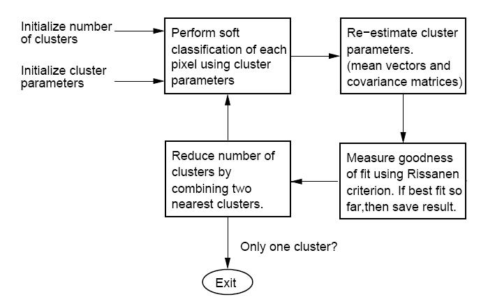
The "CLUSTER" software, developed by Purdue University's own Professor Charles Bouman, can be found, along with all supporting documentation, here: Cluster Homepage. The algorithm takes an iterative bottom-up (or agglomerative) approach to clustering. Different from many clustering algorithms, this one uses a so-called "Rissanen criterion" or "minimum description length" (MDL_OldKiwi) as the best fit criterion. In short, MDL_OldKiwi favors density estimates with parameters that may be encoded (along with the data) with very few bits. i.e. The simpler it is to represent both the density parameters and data in some binary form, the better the estimate is considered.

Note: there is a typo in the manual that comes with "CLUSTER." In the overview figure, two of the blocks have been exchanged. The figure below hopefully corrects this typo.

Below is the block diagram from the software manual (with misplaced blocks corrected) describing the function of the software. (Fig.2)

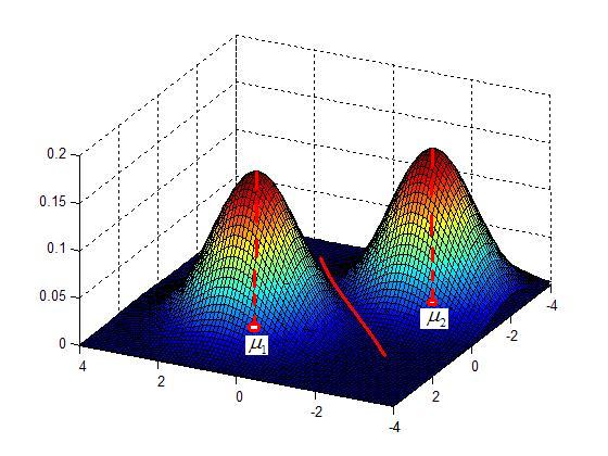
Clustering by finding valleys of densities

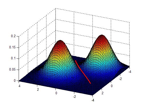
Idea: Cluster boundaries correspond to local minima of density fct (=valleys)

in 2D

(Fig.3)

Advantages

• no presumptions about the shape of the data
• no presumptions about the number of clusters

Approach 1: "bump hunting"

Reference: CLIQUE98 Agrawal et al.

• Approximate the density fct p(x), (Using Parzen window)
• Approximate the density fct p(x), (Using K-Nearest Neighbor)

References

• CLIQUE98 Agrawal et al.