Latest revision as of 10:25, 10 June 2013

ECE662: Statistical Pattern Recognition and Decision Making Processes

Spring 2008, Prof. Boutin

Slecture

Collectively created by the students in the class

Lecture 28 Lecture notes

Jump to: Outline| 1| 2| 3| 4| 5| 6| 7| 8| 9| 10| 11| 12| 13| 14| 15| 16| 17| 18| 19| 20| 21| 22| 23| 24| 25| 26| 27| 28

The Last Class

Welcome to the last class of the semester! The kiwi is going to be a great resource.

Partial Differential Equations (Continued)

[Note: I do not think the difference between $\partial$ and $$ d $$ is very important -- feel free to fix it if you disagree. I'm also a little sloppy with the vector symbols]

\frac{d}{dt}=u_{xx}

We may discretize this using a finite difference equation.

\frac{u(t+\Delta t,x)-u(t,x)}{\Delta t}=\frac{u(t,x+\Delta x)-2u(t,x)+u(t,x-\Delta x)}{\Delta x^{2}}

u(t+\Delta t,x)=u(t,x)+\frac{\Delta t}{\Delta x^{2}}(u(t,x+\Delta x)-2u(t,x)+u(t,x-\Delta x))

where $$ u(t,x) $$ is the initial guess. But we can also look at this

a different way.

=\frac{\Delta t}{\Delta x^{2}}u(t,x+\Delta x)+(1-2\frac{\Delta t}{\Delta x^{2}})u(t,x)+\frac{\Delta t}{\Delta x^{2}}u(t,x-\Delta x)

What does this mean? Let's consider an example.

We fix t, and let

\frac{\Delta t}{\Delta x^{2}}=\frac{1}{3}

. Then

u(t+\Delta t,x)=\frac{1}{3}u(t,x+\Delta x)+\frac{1}{3}u(t,x)+\frac{1}{3}u(t,x-\Delta x)

This is the same as convolution:

[Figure: [1/3,1/3,1/3]*[(x-delx),*(x),(x+delx)]u(t,.) ]

At each successive time step, the convolution iterates on the results of the previous convolution until the solution stabilizes. (That is, until we reach the steady state solution, where $\frac{du}{dt}=0\Longrightarrow u_{xx}=0$ )

We can use heat flow to smooth out parametric curves.

e.g. in

\mathbb{R}^{2}

, consider the curve

\overrightarrow{\tau}(\tau)=(x(\tau),y(\tau))

We shall commonly drop the vector notation in the rest of this discussion.

[Figure: Arbitrary curve , looping from $\tau=0$ to $\tau=10,000$ .]

And consider the family

c(t,\tau)=(x(t,\tau),y(t,\tau))

satisfying the 2D heat equation

\frac{dc}{dt}=\frac{d^{2}c}{d\tau^{2}}

This gives us two 1-D heat equations

\frac{dx}{dt}=\frac{d^{2}x}{d\tau^{2}}

\frac{dy}{dt}=\frac{d^{2}y}{d\tau^{2}}

The solution to these equations is

x(t,\tau)=x(0,\tau)*G(t,\tau)

y(t,\tau)=y(0,\tau)*G(t,\tau)

If we cannot solve these analytically, we can again discretize the solution.

x_{i,j+1}=x_{j}+\frac{\Delta t}{(\Delta\tau)^{2}}(x_{i+1,j}-2x_{i,j}+x_{i-1,j})

y_{i,j+1}=y_{j}+\frac{\Delta t}{(\Delta\tau)^{2}}(y_{i+1,j}-2y_{i,j}+y_{i-1,j})

Note that $\Delta\tau\neq\Delta x$ . $\Delta\tau$ is the spacing between the parameters, and is a constant. However, $\Delta x$ is the spacing of the points in the x direction, and it is certainly not constant around the entire curve! And a little note on notation:

x(0,0)=x_{0,0}

x(\Delta t,\Delta\tau)=x_{1,1}

x(2\Delta t,\Delta\tau)=x_{2,1}

[Figure showing the notation]

At this point in the class, we reviewed how to solve differential equations iteratively.

How does this apply to valley-finding?

Use estimated density $$ p(x) $$ to define the energy of the curve in

the feature space. The simplest formulation is

E=\int_{curve}p(c(\tau))d\tau

It's funny that rivers solve PDEs. They find the minimal energy route through the valleys. This is exactly what we want, because the valleys separate the mountains, which are our clusters.

Look for a curve that minimizes E. For example, in 2D feature space, look for a curve in $\mathrm{R}^{2}$ , say $c(\tau)=(x(\tau),y(\tau))$ ,

such that

E=\int_{curve}p(x(\tau),y(\tau))d\tau

Gradient descent from

\frac{dc}{dt}=E'

.

\frac{dc}{dt}=-\nabla p(x,y)

\frac{dx}{dt}(t,\tau)=-\frac{d}{dx}p(x,y)

\frac{dy}{dt}(t,\tau)=-\frac{d}{dx}p(x,y)

Numerically, we need to discritize the left hand side, but not the

right hand side

\frac{x(t+\Delta t,\tau)-x(t,\tau)}{\Delta\tau}=-p_{x}(x(t,\tau),y(t,\tau))

which we can rewrite as

x(t+\Delta t,\tau)=x(t,\tau)-\Delta\tau p_{x}(x(t,\tau),y(t,\tau))

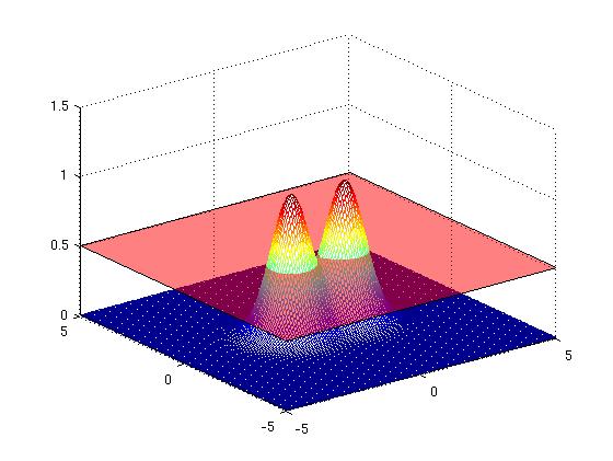
[Figure of density points and approximated density landscape.]

[Start with curve around both mountains, this is the initial guess for the boundaries of the feature space]

[Note that the curve is discritized, each point is assigned to a different value of $\tau$ ]

We can represent the points on the curve in a matrix

\left(\begin{matrix} x(1), & y(1)\\ x(2), & y(2)\\ \vdots\\ x(20) & y(20)\end{matrix}\right)

Then we can iterate using the equation above to find the boundaries which minimizes the energy, and is thus the best seperation of the clusters.

Issues with this approach

We must fix the number of clusters
We must assume the curve has some degree of smoothness.

[Figure of this phenomenon]

The points tend to collapse on each other or move away from each other.

[Figure of this phenomenon] How can we overcome these difficulties? With (as the Spanish developers might call it) "De Le-vel set." (pronounced with the long e sound which doesn't really exist in English so much.)

The Level Set Approach

This method was developed by Osher and Sethian [spelling?].

Assume we are evolving a curve in $\mathbb{R}^{2}$ . Instead of doing this, we evolve a surface in $\mathbb{R}^{3}$ for which the ``zero level set, that is the intersection with the z=0 plane is the curve we wish to evolve.

[Figure of an evolving curve]

[Figure of evolving surface instead of curve]

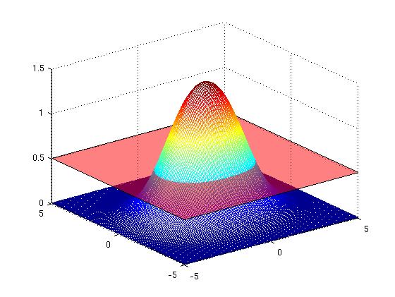
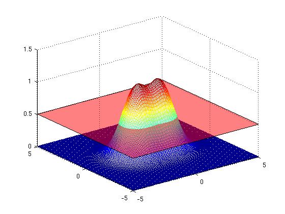
Although evolving such a surface can be challenging, it is definitely worth it, because our curve may undergo topology changes. How can this happen? Even though the surface evolves without topology changes, the zero-set (our curve) can change topologies and have singularities.

From the Dromedary (French: Dromadaire) to the Camel (French: Chameau)

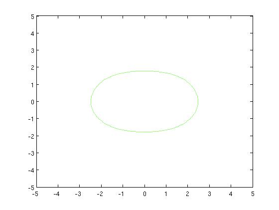
[Figure t=0: of the one-hump animal, yielding a single curve]

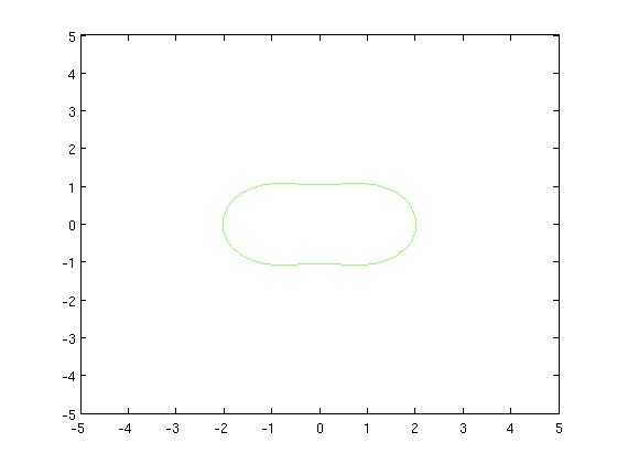
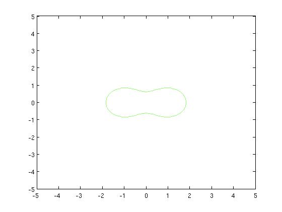
[Figure t=1: The top flattens, the curve turns into a peanut]

[Figure t=2: The valley dips so we get the Chameau]

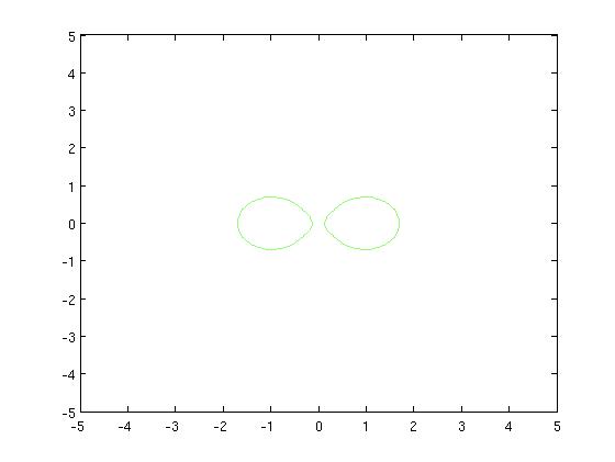
[Figure t=3: The Chameau sinks deeper in the water so that only two humps appear. The curve splits into two]

We evolve the surface until it converges, and then we can look at the resulting zero-set and count the clusters. We do not need ot know them a-priori.

As a note for those who are not taking this class: We use French here because that is the mother language of our professor (Mimi), and because we were having difficulty finding the English words for these at first! (And by "we", we do mean the entire class.)

What PDE describes this surface evolution?

Suppose

\frac{d}{dt}(x(t,\tau),y(t,\tau))=f(t,\tau)\overrightarrow{N}(t,\tau)

where $\overrightarrow{N}(t,\tau)$ is normal to the curve. This is a very general equation because any curve evolution can be expressed in this fashion. Then we can consider a surface evolving $\phi(x,y,t):=\mathbb{R}^{2}\times\mathbb{R}\rightarrow$ a zero-level set at t, $\left\{ x,y|\phi(x,y,t)=0\right\}$ is the

curve we are evolving. The Euler form of the level set is

\frac{d\phi}{dt}=f(t,\tau)||\nabla\phi||

Conclusion

And that's it for the semester! Have fun!

@@ Line 1: / Line 1: @@
+[[Category:ECE662]]
+[[Category:decision theory]]
+[[Category:lecture notes]]
 [[Category:pattern recognition]]
-[[Category:sLecture]]
+[[Category:slecture]]
 <center><font size= 4>
 '''[[ECE662]]: Statistical Pattern Recognition and Decision Making Processes'''
@@ Line 8: / Line 10: @@
 Spring 2008, [[user:mboutin|Prof. Boutin]]
-sLecture
+[[Slectures|Slecture]]
 <font size= 3> Collectively created by the students in [[ECE662:BoutinSpring08_OldKiwi|the class]]</font size>
@@ Line 15: / Line 17: @@
 ----
 =Lecture 28 Lecture notes=
-Quick link to lecture notes: [[Lecture 1 - Introduction_OldKiwi|1]]|
+Jump to: [[ECE662_Pattern_Recognition_Decision_Making_Processes_Spring2008_sLecture_collective|Outline]]|
+[[Lecture 1 - Introduction_OldKiwi|1]]|
 [[Lecture 2 - Decision Hypersurfaces_OldKiwi|2]]|
 [[Lecture 3 - Bayes classification_OldKiwi|3]]|
@@ Line 22: / Line 25: @@
 [[Lecture 6 - Discriminant Functions_OldKiwi|6]]|
 [[Lecture 7 - MLE and BPE_OldKiwi|7]]|
-[[Lecture 8 - MLE, BPE and Linear Discriminant Functions_OldKiwi|8]]
+[[Lecture 8 - MLE, BPE and Linear Discriminant Functions_OldKiwi|8]]|
 [[Lecture 9 - Linear Discriminant Functions_OldKiwi|9]]|
-[[Lecture 10 - Batch Perceptron and Fisher Linear Discriminant_OldKiwi|10]]
+[[Lecture 10 - Batch Perceptron and Fisher Linear Discriminant_OldKiwi|10]]|
 [[Lecture 11 - Fischer's Linear Discriminant again_OldKiwi|11]]|
 [[Lecture 12 - Support Vector Machine and Quadratic Optimization Problem_OldKiwi|12]]|

Difference between revisions of "Lecture 28 - Final lecture OldKiwi" - Rhea