(→Three crucial questions to answer) |
|||
| (7 intermediate revisions by 2 users not shown) | |||
| Line 1: | Line 1: | ||
| + | <center><font size= 4> | ||
| + | '''[[ECE662]]: Statistical Pattern Recognition and Decision Making Processes''' | ||
| + | </font size> | ||
| + | |||
| + | Spring 2008, [[user:mboutin|Prof. Boutin]] | ||
| + | |||
| + | [[Slectures|Slecture]] | ||
| + | |||
| + | <font size= 3> Collectively created by the students in [[ECE662:BoutinSpring08_OldKiwi|the class]]</font size> | ||
| + | </center> | ||
| + | |||
| + | ---- | ||
| + | =Lecture 21 Lecture notes= | ||
| + | Jump to: [[ECE662_Pattern_Recognition_Decision_Making_Processes_Spring2008_sLecture_collective|Outline]]| | ||
| + | [[Lecture 1 - Introduction_OldKiwi|1]]| | ||
| + | [[Lecture 2 - Decision Hypersurfaces_OldKiwi|2]]| | ||
| + | [[Lecture 3 - Bayes classification_OldKiwi|3]]| | ||
| + | [[Lecture 4 - Bayes Classification_OldKiwi|4]]| | ||
| + | [[Lecture 5 - Discriminant Functions_OldKiwi|5]]| | ||
| + | [[Lecture 6 - Discriminant Functions_OldKiwi|6]]| | ||
| + | [[Lecture 7 - MLE and BPE_OldKiwi|7]]| | ||
| + | [[Lecture 8 - MLE, BPE and Linear Discriminant Functions_OldKiwi|8]]| | ||
| + | [[Lecture 9 - Linear Discriminant Functions_OldKiwi|9]]| | ||
| + | [[Lecture 10 - Batch Perceptron and Fisher Linear Discriminant_OldKiwi|10]]| | ||
| + | [[Lecture 11 - Fischer's Linear Discriminant again_OldKiwi|11]]| | ||
| + | [[Lecture 12 - Support Vector Machine and Quadratic Optimization Problem_OldKiwi|12]]| | ||
| + | [[Lecture 13 - Kernel function for SVMs and ANNs introduction_OldKiwi|13]]| | ||
| + | [[Lecture 14 - ANNs, Non-parametric Density Estimation (Parzen Window)_OldKiwi|14]]| | ||
| + | [[Lecture 15 - Parzen Window Method_OldKiwi|15]]| | ||
| + | [[Lecture 16 - Parzen Window Method and K-nearest Neighbor Density Estimate_OldKiwi|16]]| | ||
| + | [[Lecture 17 - Nearest Neighbors Clarification Rule and Metrics_OldKiwi|17]]| | ||
| + | [[Lecture 18 - Nearest Neighbors Clarification Rule and Metrics(Continued)_OldKiwi|18]]| | ||
| + | [[Lecture 19 - Nearest Neighbor Error Rates_OldKiwi|19]]| | ||
| + | [[Lecture 20 - Density Estimation using Series Expansion and Decision Trees_OldKiwi|20]]| | ||
| + | [[Lecture 21 - Decision Trees(Continued)_OldKiwi|21]]| | ||
| + | [[Lecture 22 - Decision Trees and Clustering_OldKiwi|22]]| | ||
| + | [[Lecture 23 - Spanning Trees_OldKiwi|23]]| | ||
| + | [[Lecture 24 - Clustering and Hierarchical Clustering_OldKiwi|24]]| | ||
| + | [[Lecture 25 - Clustering Algorithms_OldKiwi|25]]| | ||
| + | [[Lecture 26 - Statistical Clustering Methods_OldKiwi|26]]| | ||
| + | [[Lecture 27 - Clustering by finding valleys of densities_OldKiwi|27]]| | ||
| + | [[Lecture 28 - Final lecture_OldKiwi|28]] | ||
| + | ---- | ||
| + | ---- | ||
When the number of categories, c is big, decision tress are particularly good. | When the number of categories, c is big, decision tress are particularly good. | ||
| Line 123: | Line 167: | ||
'''Idea''': Look further than horizon but step back if it is not worth it. | '''Idea''': Look further than horizon but step back if it is not worth it. | ||
| − | [[Image: | + | [[Image:ECE662_lect21_stopping_OldKiwi.jpg]] |
Here is an example where increasing the number of nodes typically lowers the impurity. If the stopping condition looks at at a short horizon, then the number of nodes may stop at the first stopping point. If the horizon continues, then the number of nodes can stop at the second stopping point, which appears to be the best location for this example. | Here is an example where increasing the number of nodes typically lowers the impurity. If the stopping condition looks at at a short horizon, then the number of nodes may stop at the first stopping point. If the horizon continues, then the number of nodes can stop at the second stopping point, which appears to be the best location for this example. | ||
| + | ---- | ||
| + | Previous: [[Lecture_20_-_Density_Estimation_using_Series_Expansion_and_Decision_Trees_OldKiwi|Lecture 20]] | ||
| + | Next: [[Lecture_22_-_Decision_Trees_and_Clustering_OldKiwi|Lecture 22]] | ||
| − | [[Category: | + | [[ECE662:BoutinSpring08_OldKiwi|Back to ECE662 Spring 2008 Prof. Boutin]] |
| + | [[Category:ECE662]] | ||
| + | [[Category:decision theory]] | ||
| + | [[Category:lecture notes]] | ||
| + | [[Category:pattern recognition]] | ||
| + | [[Category:slecture]] | ||
Latest revision as of 10:23, 10 June 2013
ECE662: Statistical Pattern Recognition and Decision Making Processes
Spring 2008, Prof. Boutin
Collectively created by the students in the class
Lecture 21 Lecture notes
Jump to: Outline| 1| 2| 3| 4| 5| 6| 7| 8| 9| 10| 11| 12| 13| 14| 15| 16| 17| 18| 19| 20| 21| 22| 23| 24| 25| 26| 27| 28
When the number of categories, c is big, decision tress are particularly good.
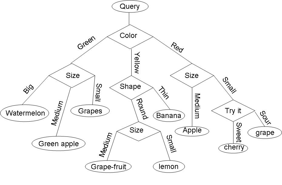
Example: Consider the query "Identify the fruit" from a set of c=7 categories {watermelon, apple, grape, lemon, grapefruit, banana, cherry} .
One possible decision tree based on simple queries is the following:
Three crucial questions to answer
How do you grow or construct a decision tree using training data?
CART Methodology - Classification and Regressive Tree
For constructing a decision tree, for a given classification problem, we have to answer these three questions
1) Which question should be asked at a given node -"Query Selection"
2) When should we stop asking questions and declare the node to be a leaf -"When should we stop splitting"
3) Once a node is decided to be a leaf, what category should be assigned to this leaf -"Leaf classification"
We shall discuss questions 1 and 2 (3 being very trivial)
Need to define 'impurity' of a dataset such that $ impurity = 0 $ when all the training data belongs to one class.
Impurity is large when the training data contain equal percentages of each class
$ P(\omega _i) = \frac{1}{C} $; for all $ i $
Let $ I $ denote the impurity. Impurity can be defined in the following ways:
Entropy Impurity:
$ I = \sum_{j}P(\omega _j)\log_2P(\omega _j) $, when priors are known, else approximate $ P(\omega _j) $ by $ P(\omega _j) = \frac{\#\,of\,training\,patterns\,in\,\omega_j}{Total\,\#\,of\,training\,patterns} $
Gini Impurity
$ I = \sum_{i\ne j}P(\omega _i)P(\omega _j) = \frac{1}{2}[1- \sum_{j}P^2(\omega _j) $
Ex: when C = 2, $ I = P(\omega _1)P(\omega _2) $
Misclassification Impurity
$ I = 1-max P(\omega _j) $
defined as the "minimum probability that a training pattern is misclassified"
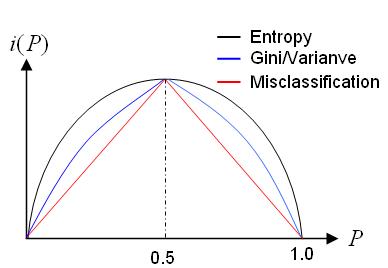
The following figure shows above-mentioned impurity functions for a two-category case, as a function of the probability of one of the categories.(DHS-399p)
Now let us look at each of the three questions in detail.
Query Selection
Heuristically, want impurity to decrease from one node to its children.
We assume that several training patterns are available at node N and they have a good mix of all different classes.
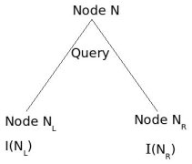
I(N) := impurity at node N.
Define impurity drop at node N as: $ \triangle I=I(N)-P_{L}I(N_{L})-(1-P_{L})I(N_{R}) $
where $ P_{L} $ and $ (1-P_{L}) $ are estimated with training patterns at node N.
A query that miximizes $ \triangle I $ is "probably" a good one. But "finding the query that maximizes" is not a well defined question because we are not doing an exhaustive search over all the possible queries. Rather we narrow down to a set of few queries and find among them, which one maximizes $ \triangle I $.
Example:
1. look at separation hyperplane that miximizes $ \triangle I(N) $
2. look for a single feature threshold (colour or shape or taste) which would maximize $ \triangle I(N) $
Query selection => numerical optimization problem.
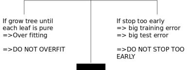
When to stop splitting ?
Key: look for balance.
Need to construct a "balanced tree". Many ways to do this.
Example:
1. Validation - train with 80% of training data, validate on 20%. Continue splitting until validation error is minimized.
2. Thresholding - stop splitting when threshold $ \beta $ is small (but not too small)
$ \beta=0.03 $
Warning: "Horizon Effect"
Lack of looking ahead may cause us to stop splitting prematurely.
You should keep splitting for a bit, after you meet stopping criteria.
How to correct oversplitting?
Use "pruning" (or inverse splitting) which implies that take 2 leaves that have a common parent and merge them if "merging helps" i.e.
- if I either doesn't change or only increases a little bit.
- if validation error either stays the same or decreases.
Declare parent to be a leaf.
Pruning increases generalization.
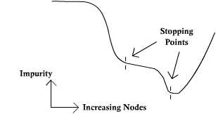
Idea: Look further than horizon but step back if it is not worth it.
Here is an example where increasing the number of nodes typically lowers the impurity. If the stopping condition looks at at a short horizon, then the number of nodes may stop at the first stopping point. If the horizon continues, then the number of nodes can stop at the second stopping point, which appears to be the best location for this example.
Previous: Lecture 20 Next: Lecture 22

