Table of Contents:
- Introduction
- Basic Understanding
- Deeper Understanding and Example
- Applications
- References
Introduction:
Singular Value Decomposition has many names, such as factor analysis, empirical orthogonal function analysis, and principal component decomposition. In this discussion, I will refer to it as SVD. To put it simply, Singular Value Decomposition is decomposing a singular matrix into three parts so that it is easier to understand and transform. This has many applications in data science when displaying a set of information in a matrix. SVD is mainly used in linear algebra, but it can be understood in its most basic form as early as Calculus or even in Physics classes when breaking down vectors into components and projections. SVD was discovered by many different mathematicians in the late 1800s, namely Eugenio Beltrami and Camille Jordan, but would later become very important with the development of computers and big data.
Basic Understanding:
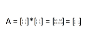
Before we get into what SVD really means, it is important to understand some basic concepts. Firstly, SVD deals with matrices, which are a collection of values put into rows and columns. Matrices can be described by the number of rows (n) and columns (m) that they have in the form n x m, which is important to understand when performing operations on them. Matrices can be added, subtracted, multiplied, and divided just like functions, but the processes are a little different. For example, to multiply a matrix by another, you must take the dot product of the two. This is when you multiply each value in the row of the first matrix by each value in the column of the second matrix. For example:
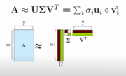
Additionally, to divide matrices, you are actually multiplying by the inverse. However, this is not as important when it comes to SVD. The main equation for SVD is A=USV^T, where: “A is an m × n matrix, U is an m × n orthogonal matrix, S is an n × n diagonal matrix, and V is an n × n orthogonal matrix,” (1). An orthogonal matrix is when the columns and rows are perpendicular unit vectors, and a diagonal matrix contains all values that are zero except in the diagonal line down from the top left to the bottom right. Additionally, in the equation, the ^T stands for “transpose” of the matrix which basically flips the original matrix. We know that U^TU and V^TV both give the identity matrix because U and V are orthogonal. Another way of viewing this equation is by looking at it graphically: (7)
Going Deeper:
To gain a better understanding of how we can use SVD, let’s look at an example from the video about Singular Value Decomposition from Stanford University. In the example, there is a data set of 7 people and 5 different movies that they watched. Each person rated each movie, and the matrix arranges this data to show who liked which movie. From the movie options, we can see that there were two main genres of movies watched- Romance and Sci-Fi. By taking the SVD to analyze this data, we find this output: The first matrix U represents how each person responded to the different genres, where the first column represents the Sci-Fi genre and the second relates to the Romance concept. We can see that the first four people responded more strongly to the Sci-Fi genre as there is a higher correlation in that matrix, while the last three more towards Romance. The second diagonal matrix S shows the strength of each genre, or how many people liked it. So, Sci-Fi was the most popular genre because it has a strength of 12.4. The last value (1.3) shows that the third column does not have a large strength on the data, so it does not represent a significant genre and we can ignore it. The last matrix V relates to how strongly each movie corresponds to the two concepts. From this, we can see that “Casablanca” and “Amelie” are more strongly related to romance, while the other three movies are closer to the Sci-Fi category. So, by using SVD we can learn more about each individual person and their preferences for the movies as well as how the movies relate to each genre presented.


