Multivariate Normal Density

Because of the mathematical tractability as well as because of the central limit theorem, Multivariate Normal Density, as known as Gaussian Density, received more attention than other various density functions that have been investigated in pattern recognition.

The general multivariate normal density in d dimensions is:

where

$ \mathbf{x}=[x_1,x_2,\cdots ,x_d]^t $ is a d-component column vector,

$ \mathbf{\mu}=[\mu_1,\mu_2,\cdots ,\mu_d]^t $ is the d-component mean vector,

$ \mathbf{\Sigma}=\begin{bmatrix} \sigma_1^2 & \cdots & \sigma_{1d}^2\\ \vdots & \ddots & \\ \vdots \sigma_{d1}^2 & \cdots & \sigma_d^2 \end{bmatrix} $ is the d-by-d covariance matrix,

$ |\mathbf{\Sigma|} $ is its determinant,

$ \mathbf{\Sigma}^{-1} $ is its inverse.

Each $ p(x_i)\sim N(\mu_i,\sigma_i^2) $, so $ \Sigma $ plays role similar to the role that $ \sigma^2 $ plays in one dimension. Thus, we can find out the relationship among different features (such as $ x_i $ and $ x_j $)through $ \Sigma $:

• $ \sigma_{ij}=0 $, $ x_i $ and $ x_j $ are independent;
• $ \sigma_{ij}>0 $, $ x_i $ and $ x_j $ are positive correlated;
• $ \sigma_{ij}<0 $, $ x_i $ and $ x_j $ are negative correlated.

Discriminant Functions

One of the most useful method to represent pattern classifiers is in terms of a set of discriminant functions $ g_i(\mathbf{x}), i=1,2,...,c $. The classifier is said to assign a feature vector $ \mathbf{x} $ to class $ w_i $ if

Thus, the classification is viewed as process to compute the discriminant functions and select the category corresponding to the largest discriminant. A Bayes classifier is easily represented in this way. In order to simplify the classification process, minimum-error-rate classification is always chosen by taking $ g_i({\mathbf{x}}) $ in natural logarithm format:

Equation (2) can be readily evaluated if the densities $ p(\mathbf{x}|w_i) \sim N(\mathbf{\mu}_i, \mathbf{\Sigma}_i) $. From Equation (1), we have the following discriminant function for multivariate normal density:

we will use Equation (3) to discuss three special classification cases in the next part. To point out that, in next part, two classes two dimension features will be used in the discussion.

Classification for Three Special Cases

Case 1:

$ \mathbf{\Sigma}_i = \sigma^2 \mathbf{I} $

In this case, features $ x_1 $ $ x_2 $ are independent with different means and equal variances. That is,

Thus, $ \mathbf{\Sigma}_i^{-1}=1/\sigma^2 $ and $ \mathbf{\Sigma}_i $ is a constant. So the discriminant function shown in Equation (3) can be simplified to Equation (4):

Expand Equation (4), we obtain

Since $ \mathbf{x}^t \mathbf{x} $ is a constant for all classes, so we can expand Equation (5) continuously,

Since $ \frac{\mathbf{\mu}_i^t}{\sigma^2} $ and $ -\frac{\mathbf{\mu}_i^t \mathbf{\mu}_i}{2 \sigma^2}+\ln P(w_i) $ are constant in $ \mathbf{x} $, so if we let $ w_i=\frac{\mathbf{\mu}_i^t}{\sigma^2} $, $ w_{i0}=-\frac{\mathbf{\mu}_i^t \mathbf{\mu}_i}{2 \sigma^2}+\ln P(w_i) $, we obtain

Thus, from Equation (7), we conclude that in Case 1, the classifier is a linear classifier.

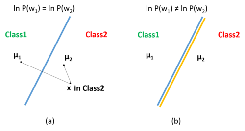
Figure 1 shows the geometric interpretation of Case 1: if the prior probabilities $ P(w_i) $ are the same for all classes, to classify a feature vector $ x $, we just should assign it to the category of the nearest mean, as shown in (a); if the prior probabilities $ P(w_i) $ are not the same for all classes, the decision boundary shifts away from the more likely mean, as shown in (b).

Figure 1. Geometric Interpretation of Case 1: (a) two classes have the same prior probability; (b) two classes do not have the same prior probabilities.

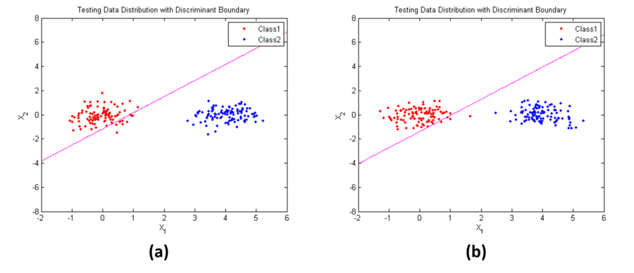
Figure 2 shows an example of Case 1. Parameters used here are:

$ \mathbf{\mu_1}=[0,3]^t $,

$ \mathbf{\mu_2}=[4,0]^t $,

$ \mathbf{\Sigma}_1=\mathbf{\Sigma}_2=\begin{bmatrix} 0.3 & 0\\ 0 & 0.3 \end{bmatrix} $

in (a), $ P(w_1)=P(w_2)=0.5 $; while in (b), $ P(w_1)= 0.1, P(w_2)=0.9 $. From the results, we find that when the prior probabilities are not the same, the position of the decision boundary is relatively insensitive (discriminant line is rotate in the counter clock direction a little bit).

Figure 2. Example of Case 1: (a) two classes have the same prior probability; (b) Class2 has a higher prior probability.

Case 2:

$ \mathbf{\Sigma}_i = \mathbf{\Sigma} $

In this case, features $ x_1 $ $ x_2 $ are not necessary independent. Though covariance matrices are equal, they are arbitrary. That is,

Thus, $ \mathbf{\Sigma}_i $ is a constant. So the discriminant function shown in Equation (3) can be simplified to Equation (8):

Expand Equation (8), we obtain

Since $ \mathbf{x}^t \mathbf{\Sigma^{-1}} \mathbf{x} $ is a constant for all classes, so we can simplifies Equation (9) continuously,

Since $ \mathbf{\mu}_i^t \mathbf{\Sigma^{-1}} \mathbf{x} $ and $ \ln P(w_i)-\frac{1}{2}\mathbf{\mu}_i^t \mathbf{\Sigma^{-1}} \mathbf{\mu}_i $ are constant in $ \mathbf{x} $, so if we let

$ w_i=\mathbf{\mu}_i^t \mathbf{\Sigma^{-1}} \mathbf{x} $,

$ w_{i0}=\ln P(w_i)-\frac{1}{2}\mathbf{\mu}_i^t \mathbf{\Sigma^{-1}} \mathbf{\mu}_i $,

we obtain

Thus, from Equation (11), we conclude that in Case 2, the classifier is also a linear classifier.

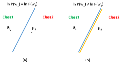
Figure 3 shows the geometric interpretation of Case 2: if the prior probabilities $ P(w_i) $ are the same for all classes, feature vector $ x $ in each cell are closer to the mean in that cell tan to any other mean under Mahalanobis distance, as shown in (a); if the prior probabilities $ P(w_i) $ are not the same for all classes, the decision boundary shifts away from the more likely mean, as shown in (b).

Figure 3. Geometric Interpretation of Case 2: (a) two classes have the same prior probability; (b) two classes do not have the same prior probabilities.

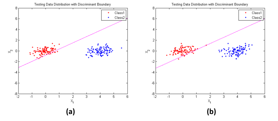
Figure 4 shows an example of Case 2. Parameters used here are:

$ \mathbf{\mu_1}=[0,3]^t $,

$ \mathbf{\mu_2}=[4,0]^t $,

$ \mathbf{\Sigma}_1=\mathbf{\Sigma}_2=\begin{bmatrix} 0.3 & 0.1\\ 0.1 & 0.3 \end{bmatrix} $

in (a), $ P(w_1)=P(w_2)=0.5 $; while in (b), $ P(w_1)= 0.1, P(w_2)=0.9 $. From the results, we also find that the position of the decision boundary is relatively insensitive when the prior probabilities are not the same.

Figure 4. Example of Case 2: (a) two classes have the same prior probability; (b) Class2 has a higher prior probability.

Case 3:

$ \mathbf{\Sigma}_i = \mathbf{arbitrary} $

In this case, features $ x_1 $ $ x_2 $ are not necessary independent and covariance matrices are arbitrary.

The discriminant function shown in Equation (3) can be simplified, but let us rearrange it:

Let

$ W_i=-\frac{1}{2}\mathbf{\Sigma}_i^{-1} $,

$ w_{i}=\mathbf{\Sigma}_i^{-1}\mathbf{\mu}_i) $,

$ w_{i0}=-\frac{1}{2}\mathbf{\mu}_i^t \mathbf{\Sigma_i^{-1}} \mathbf{\mu}_i)-\frac{1}{2}\ln |\mathbf{\Sigma}_i|+\ln P(w_i) $

we obtain

Thus, from Equation (12), we observe that the discriminant function is quadratic, so the decision boundaries are quadratic as well. Therefore, the classifier is a ellipses and parabolloids classifier.

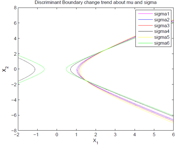
Figure 5 shows that if $ ||\Sigma_1-\Sigma_2|| $ is small relative to the distance of $ ||\mu_1-\mu_2|| $, then the position of the decision boundary is relatively insensitive to the exact values of the prior probabilities.

Figure 5. Relationship between discriminant boundary and data features.

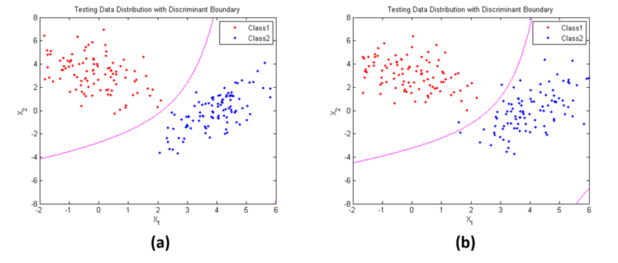
Figure 6 shows an example of Case 3. Parameters used here are:

$ \mathbf{\mu_1}=[0,3]^t $,

$ \mathbf{\mu_2}=[4,0]^t $,

$ \mathbf{\Sigma}_1=\begin{bmatrix} 1 & -0.5\\ -0.5 & 2 \end{bmatrix} $

$ \mathbf{\Sigma}_2=\begin{bmatrix} 1 & 1.2\\ 1.2 & 3 \end{bmatrix} $

in (a), $ P(w_1)=P(w_2)=0.5 $; while in (b), $ P(w_1)= 0.1, P(w_2)=0.9 $. We can see the decision boundary shape is parabolloids.

Figure 6. Example of Case 3: (a) two classes have the same prior probability; (b) Class2 has a higher prior probability.

Summary

• If covariance matrices are equal and proportional to identity matrix, the Bayes classifier is linear.

• If covariance matrices are equal, the Bayes classifier is linear.

• If covariance matrices are arbitrary, the Bayes classifier is ellipses or parabolloid.

References

1. Richard O. Duda, Peter E. Hart, and David G. Stork. 2000. Pattern Classification (2nd Edition). Wiley-Interscience.
2. Sergios Theodoridis, Aggelos Pikrakis, Konstantinos Koutroumbas, and Dionisis Cavouras. 2010. Introduction to Pattern Recognition. Elsevier Inc.
3. Keinosuke Fukunaga. 1990. Introduction to Statistical Pattern Recognition (2nd Ed.). Academic Press Prof., Inc., San Diego, CA, USA.
4. Mireille Boutin, "ECE662: Statistical Pattern Recognition and Decision Making Processes," Purdue University, Spring 2014.

Questions and comments

If you have any questions, comments, etc. please post them on this page.