Audio Signal Processing with Down-sampler and LPF Investigate

                                                                      ABSTRACT

This document is investigating the effectiveness of a LPF, (low-pass-filter) when down-sampling. We are going to down-sample various types of audio signals with down-samplers which have different down-sampling rate.

                                                                  INTRODUCTION

Formally, down-sampling can be written as

        y[n]=x[Mn]

In the frequency domain, we will have

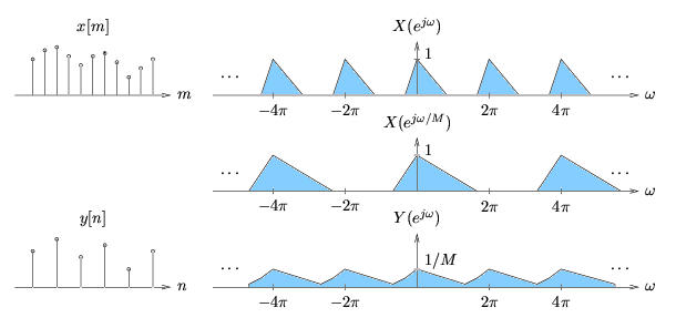
The following figure could illustrate the reason of aliasing in down-sampling.

This Figure is done by Phil Schniter.

In this project, we are going to discuss how much the LPF will help in the audio signal down-sampling.

                                                                  PROCEDURE

PART I.

In the first part of this project, we are going to develop the LPF effect to different down-sampling rates of 4, 8, and 16. In this project we are using FIR (finite impulse response) filter.
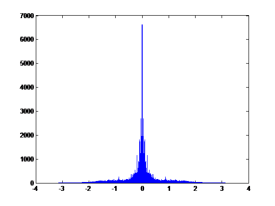
The audio signal we use is part of Waving Flag, the theme song of 2010 South Africa World Cup. We choose this signal because that this sound includes clear mix of human voice and sound of instruments.

The sound of original signal: projectrhea.org/rhea/images/f/f3/Flag.wav
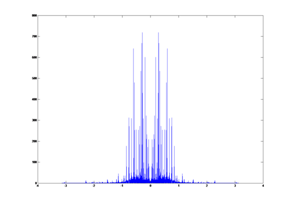
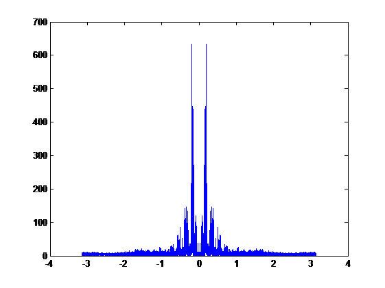
The DFT of original signal:

1. Down-sampling rate of 4:

Without using a LPF filter, the down-sampling signal: projectrhea.org/rhea/images/2/26/Flag4.wav

                           
By using the LPF filter (Gain = 1 and Cut-off frequency = π/4), the down-sampling signal: projectrhea.org/rhea/images/1/16/Flag4f.wav

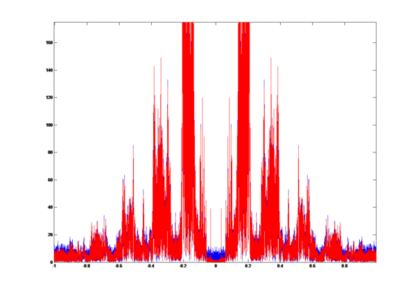
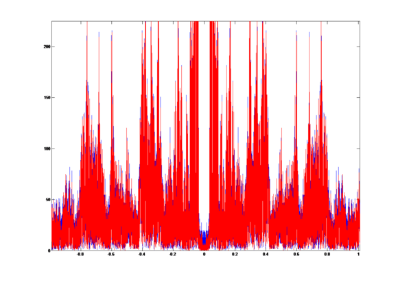
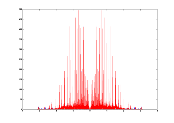
To compare the two signals above, we get the overlap graph:

The blue plot is the signal without LPF and the red plot is the signal with LPF. We can easily find the aliasing part in the graph.

Compute the correlation coefficient r = 0.9958.

 2. Down-sampling rate of 8:

Signal without LPF: projectrhea.org/rhea/images/6/65/Flag8.wav 

Signal with LPF: projectrhea.org/rhea/images/2/2e/Flag8f.wav

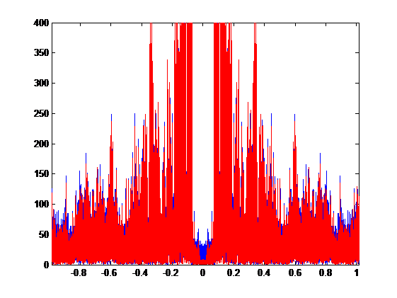
Compare the two signals, we get the overlap graph:

The blue plot is the signal without LPF and the red plot is the signal with LPF. 

Compute the correlation coefficient r = 0.9744.

3. Down-sampling rate of 16:

Signal without LPF: projectrhea.org/rhea/images/a/a3/Flag16.wav

Signal with LPF: projectrhea.org/rhea/images/7/7d/Flag16f.wav

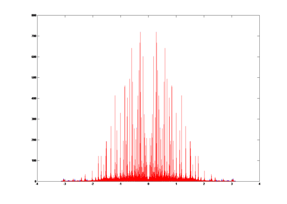
Compare the down-sampling signals with and without LPF, we get the overlap graph: 

The blue plot is the signal without LPF and the red plot is the signal with LPF.

Compute the correlation coefficient r = 0.9475.

Conclusions and finds of Part I:

1. When we really hear the signal, the LPF is more effective when down-sampling rate will not cause the source sound distorted. The audio signal we input, which is MP3 sound quality, is a human voice which is sampled at 44,100 Hz. The typical human voice frequency ranges from about 60 to 7,000 Hz. In this project, a down-sampling rate larger than 6 will weaken the function of LPF. So if we already distorted the signal when we down-sampling it, the LPF is less effective.
2. From the correlation coefficients, we can see that the correlation coefficients are decreasing when sampling rate increased. The correlation coefficients may not relate to the similarity of two sounds.

PART II:

In the second part of this project, we will repeat the same procedures in PART I, but instead of using a human voice, we will use sound from piano. The piece we choose is Figlio Perduto, the Second Movement from Symphony No. 7 by Ludwig Van Beethoven.

The sound of original signal: projectrhea.org/rhea/images/4/4f/Per.wav

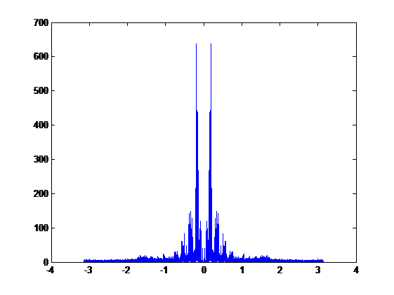
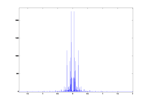
The DFT of original signal is:
                         

1. Down-sampling rate of 4:

Without using a LPF filter, the down-sampling signal: projectrhea.org/rhea/images/c/cf/Per4.wav
                           

By using the LPF filter (Gain = 1 and Cut-off frequency = π/4), the down-sampling signal: projectrhea.org/rhea/images/9/9a/Per4f.wav

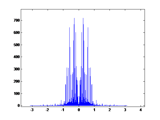
Compare the two signals above, we get the overlap graph:

The bule plot is the signal without LPF and the red plot is the signal with LPF. We can hardly see any difference between these two signals.

2. Down-sampling rate of 8:

Signal without LPF: projectrhea.org/rhea/images/a/a1/Per8.wav

Signal with LPF: projectrhea.org/rhea/images/b/ba/Per8f.wav

Compare the two signals, we get the overlap graph;

The blue plot is signal without LPF and the red plot is signal with LPF. We still can't see much difference here.

Conclusions and finds of PART II:

1. From comparing this plot and the DFT of Waving the Flag, we can see that the signal of music instruments have clear gaps between each peak and concentrate on some specific frequency. However the signal of human voice is more spread on the frequency plot.
2. Music instrument signals are less affected by LPF. From the overlap graph, we can see that these two plots overlapped each other. Also, if we play the piece, we can hear no difference between the two. So for down sampling a instrument music signal, the LPF actually makes no much difference.