Audio Signal Processing with Down-sampler and LPF Investigate

                                                                      ABSTRACT

A LPF (low-pass-filter) will usually be used before down-sampling to reduce aliasing. In this document, we investigated the effect of the LPF by comparing the difference in frequency domain and human ear perception of the signal with/without passing though a LPF before down-sampling. In the first part of this document, we down-sampled a signal of human voice with rates of 4, 8, and 16 with/without corrrespondinng LPFs. The effect of the LPF is weakening while the down-sampling rate is increasing. In the second part, we applied the same procedures in part I to a piano song. The effect of the LPF is less noticeable compared with human voice signal.

                                                                  INTRODUCTION

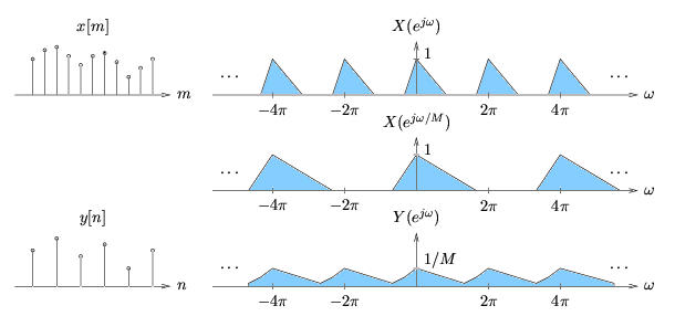
Formally, down-sampling can be written as

        y[n]=x[Mn]

In the frequency domain, we will have

The following figure could illustrate the reason of aliasing in down-sampling.

This Figure is done by Phil Schniter.

In this project, we are going to discuss how much the LPF will help in the audio signal down-sampling.

Further information about down-sampling rate can reference this particle: Sample Rate Convertion.

                                                                  PROCEDURE

PART I.

In the first part of this project, we are going to develop the LPF effect to different down-sampling rates of 4, 8, and 16. In this project we are using FIR (finite impulse response) filter.
The audio signal we use is part of Waving Flag, the theme song of 2010 South Africa World Cup. We choose this signal because that this sound includes clear mix of human voice and sound of instruments.

The sound of original signal: projectrhea.org/rhea/images/f/f3/Flag.wav
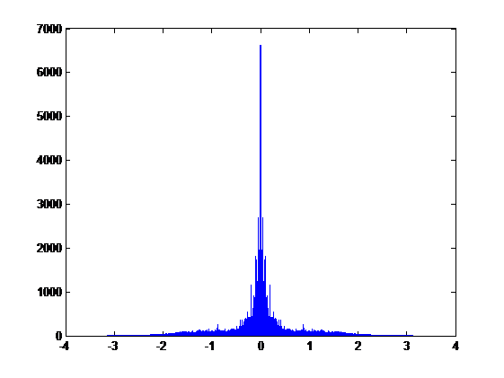
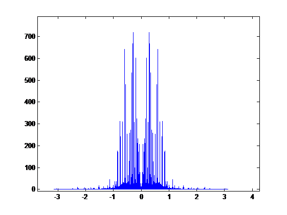
The DFT of original signal:

1. Down-sampling rate of 4:

Without using a LPF filter, the signal is down-sampled by 4.

The down-sampled signal is projectrhea.org/rhea/images/2/26/Flag4.wav.

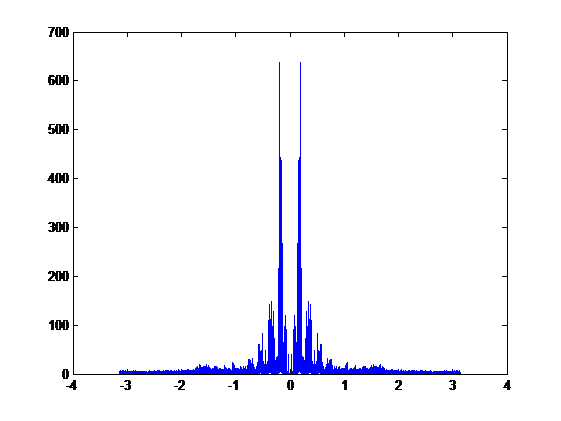
The DFT of the down-sampled signal is:

                           
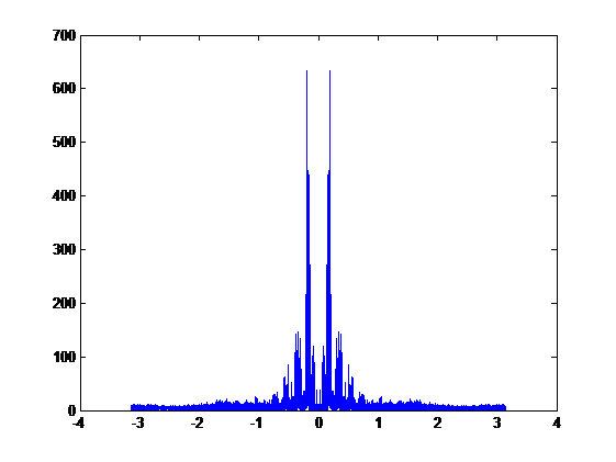
Then we use a LPF filter (Gain = 1 and Cut-off frequency = π/4) before down-sampling, the down-sampled signal: projectrhea.org/rhea/images/1/16/Flag4f.wav.

The DFT of the down-sampled signal after using a LPF is:

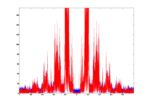
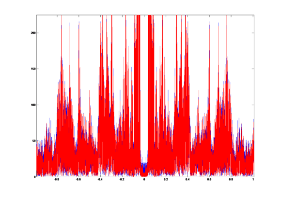
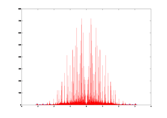
To compare the two signals above in frequency domain, we get the overlap graph:

The blue plot is the signal without LPF and the red plot is the signal with LPF. We can easily find the aliasing part in the graph.

The sampling rate for human voice is usually 8000 Hz, and the sound source we are using is sampled at 44.1K Hz. The LPF improves the down-sampling process obviously.

The blue part in the middle near 0 should be caused by the FIR filter because FIR filter has ripples in the passband.

In order to get the similarity of the two signals, we compute the correlation coefficient r = 0.9958.

 2. Down-sampling rate of 8:

The signal is down-sampled by 8 in this step. The  LPF we are using is (Gain = 1 and Cut-off frequency = π/8).

Signal down-sampled without using LPF: projectrhea.org/rhea/images/6/65/Flag8.wav 

Signal down-sampled after using LPF: projectrhea.org/rhea/images/2/2e/Flag8f.wav

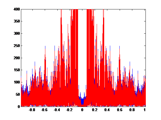
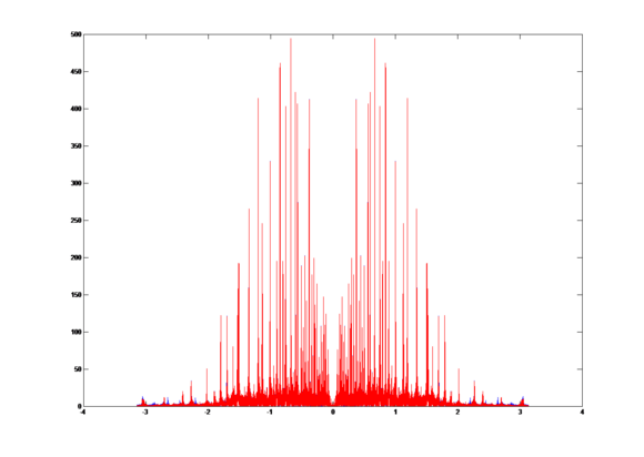
Compare the two signals in frequency domain, we get the overlap graph:

The blue plot is the signal without LPF and the red plot is the signal with LPF.

The correlation coefficient r = 0.9744.

3. Down-sampling rate of 16:

The signal is down-sampled by 16 in this step.The LPF we are using is (Gain = 1 and Cut-off frequency = π/16).

Signal down-sampled without using LPF: projectrhea.org/rhea/images/a/a3/Flag16.wav

Signal down-sampled after using LPF: projectrhea.org/rhea/images/7/7d/Flag16f.wav

Compare the down-sampling signals with and without LPF in frequency domain, we get the overlap graph: 

The blue plot is the signal without LPF and the red plot is the signal with LPF.

Compute the correlation coefficient r = 0.9475.

Conclusions and finds of Part I:

1. When playing the signal, we can hear noticeable effect of the LPF when down-sampling rate is low because the LPF is more effective when down-sampling rate will not cause the source sound distorted. The audio signal we input, which is MP3 sound quality, is a human voice which is sampled at 44,100 Hz. The typical human voice frequency ranges from about 60 to 7,000 Hz. In this project, a down-sampling rate larger than 6 will weaken the effect of LPF.

2. The difference in frequency domain is not obvious, but we still can see that the difference between red part(using LPF) and blue part(without using LPF) is decreasing. The result is consistent with what we hear.

3. From the correlation coefficients, we can see that the correlation coefficients are decreasing when sampling rate increasing. This opposes the previous findings. So the correlation coefficients of sound signals in frequency domain may not be able to show the effect of the LPF.

PART II:

In the second part of this project, we will repeat the same procedures in PART I, but instead of using a human voice, we will use sound from piano. The piece we choose is Figlio Perduto, the Second Movement from Symphony No. 7 by Ludwig Van Beethoven. We will test the effect of the LPF when down-sampling sound signal from piano and compare the result with what we get in PART I.

The sound of original signal: projectrhea.org/rhea/images/4/4f/Per.wav

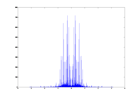
The DFT of original signal is:
                         

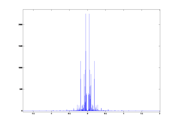
This part of the music is CD quality and is sampled by 44.1K Hz.

1. Down-sampling rate of 4:

Without using a LPF filter, the signal is down-sampled by 4.

The down-sampled signal is: projectrhea.org/rhea/images/c/cf/Per4.wav

The DFT of the down-sampled signal is:

Then we use a LPF filter (Gain = 1 and Cut-off frequency = π/4) before down-sampling, the down-sampled signal is: projectrhea.org/rhea/images/9/9a/Per4f.wav

The DFT of the down-sampled signal after using a LPF is:

Compare the two signals above in frequency domain, we get the overlap graph:

The bule plot is the signal without LPF and the red plot is the signal with LPF. We can hardly see any difference between these two signals in frequency domain.

2. Down-sampling rate of 8:

The signal is down-sampled by 8 in this step. The LPF we are using is (Gain = 1 and Cut-off frequency = π/8).

Signal down-sampled without using LPF: projectrhea.org/rhea/images/a/a1/Per8.wav

Signal down-sampled after using LPF: projectrhea.org/rhea/images/b/ba/Per8f.wav

Compare the two signals in frequency domain, we get the overlap graph:

The blue plot is signal without LPF and the red plot is signal with LPF. We still can't see much difference here.

Conclusions and finds of PART II:

1.Music instrument signals are less affected by LPF. From the overlap graph, we can see that these two plots overlapped each other. Also, if we play the piece, we can hear noticeable difference between the two. So for down-sampling a instrument music signal, the LPF actually makes no much difference. In the progress of down-sampling music piece by piano, we found that it is hard to notice the difference between signal with or without using LPFs. This mathes what we can see in the plots in frequency domain.

2.The signal of human voice is more spread on the frequency plot. In PART I, LPF is effective when down-sampling rate is 4 and is less effective when down-sampling rate is 8. The effect of LPF to aliasing we found in PART I is not appeared in PART II. From comparing the DFT plot in PART I and PART II, we can see that the signal of music instruments have clear gaps between each peak and concentrate on some specific frequency.