Contents
Lecture Objective
- Maximum Likelihood Estimation and Bayesian Parameter Estimation
- Parametric Estimation of Class Conditional Density
See also: Comparison of MLE and Bayesian Parameter Estimation_OldKiwi
The class conditional density $ p(\vec{x}|w_i) $ can be estimated using training data. We denote the parameter of estimation as $ \vec{\theta} $. There are two methods of estimation discussed.
MLE Maximum Likelihood Estimation_OldKiwi
BPE Bayesian Parameter Estimation_OldKiwi
Maximum Likelihood Estimation
Let "c" denote the number of classes. D, the entire collection of sample data. $ D_1, \ldots, D_c $ represent the classification of data into classes $ \omega_1, \ldots, \omega_c $. It is assumed that: - Samples in $ D_i $ give no information about the samples in $ D_j, i \neq j $, and - Each sample is drawn independently.
Example: The class conditional density $ p(\vec{x}|w_i) $ depends on parameter $ \vec{\theta_i} $. If $ X ~ N(\mu,\sigma^2) $ denotes the class conditional density; then $ \vec{\theta}=[\mu,\sigma^2] $.
Let n be the size of training sample, and $ D=\{\vec{X_1}, \ldots, \vec{X_n}\} $. Then,
$ p(\vec{X}|\omega_i,\vec{\theta_i}) $ equals $ p(\vec{X}|\vec{\theta}) $ for a single class.
The Likelihood Function is, then, defined as $ p(D|\vec{\theta})=\displaystyle \prod_{k=1}^n p(\vec{X_k}|\vec{\theta}) $, which needs to be maximized for obtaining the parameter.
Since logarithm is a monotonic function, maximizing the Likelihood is same as maximizing log of Likelihood which is defined as
$ l(\vec{\theta})=log p(D|\vec{\theta})=\displaystyle log(\prod_{k=1}^n p(\vec{X_k}|\vec{\theta}))=\displaystyle \sum_{k=1}^n log(p(\vec{X_k}|\vec{\theta})) $.
"l" is the log likelihood function.
Maximize log likelyhood function with respect to $ \vec{\theta} $
$ \rightarrow \hat{\theta} = argmax \left( l (\vec{\theta}) \right) $
If $ l(\vec{\theta}) $ is a differentiable function
Let $ \vec{\theta} = \left[ \theta_1, \theta_2, \cdots , \theta_p \right] $ be 1 by p vector, then
$ \nabla_{\vec{\theta}} = \left[ \frac{\partial}{\partial\theta_1} \frac{\partial}{\partial\theta_2} \cdots \frac{\partial}{\partial\theta_p} \right]^{t} $
Then, we can compute the first derivatives of log likelyhood function,
$ \rightarrow \nabla_{\vec{\theta}} ( l (\vec{\theta}) ) = \sum_{k=1}^{n} \nabla_{\vec{\theta}} \left[ log(p(\vec{x_k} | \vec{\theta})) \right] $
and equate this first derivative to be zero
$ \rightarrow \nabla_{\vec{\theta}} ( l (\vec{\theta}) ) = 0 $
Example of Guassian case
Assume that covariance matrix are know.
$ p(\vec{x_k} | \vec{\mu}) = \frac{1}{ \left( (2\pi)^{d} |\Sigma| \right)^{\frac{1}{2}}} exp \left[ - \frac{1}{2} (\vec{x_k} - \vec{\mu})^{t} \Sigma^{-1} (\vec{x_k} - \vec{\mu}) \right] $
Step 1: Take log
$ log p(\vec{x_k} | \vec{\mu}) = -\frac{1}{2} log \left( (2\pi)^d |\Sigma| \right) - \frac{1}{2} (\vec{x_k} - \vec{\mu})^{t} \Sigma^{-1} (\vec{x_k} - \vec{\mu}) $
Step 2: Take derivative
$ \frac{\partial}{\partial\vec{\mu}} \left( log p(\vec{x_k} | \vec{\mu}) \right) = \frac{1}{2} \left[ (\vec{x_k} - \vec{\mu})^t \Sigma^{-1}\right]^t + \frac{1}{2} \left[ \Sigma^{-1} (\vec{x_k} - \vec{\mu}) \right] = \Sigma^{-1} (\vec{x_k} - \vec{\mu}) $
Step 3: Equate to 0
$ \sum_{k=1}^{n} \Sigma^{-1} (\vec{x_k} - \vec{\mu}) = 0 $
$ \rightarrow \Sigma^{-1} \sum_{k=1}^{n} (\vec{x_k} - \vec{\mu}) = 0 $
$ \rightarrow \Sigma^{-1} \left[ \sum_{k=1}^{n} \vec{x_k} - n \vec{\mu}\right] = 0 $
$ \Longrightarrow \hat{\vec{\mu}} = \frac{1}{n} \sum_{k=1}^{n} \vec{x_k} $
This is the sample mean for a sample size n.
MLE Examples: Exponential and Geometric Distributions_OldKiwi
MLE Examples: Binomial and Poisson Distributions_OldKiwi
Advantages of MLE:
- Simple
- Converges
- Asymptotically unbiased (though biased for small N)
Bayesian Parameter Estimation
For a given class, let $ x $ be feature vector of the class and $ \theta $ be parameter of pdf of $ x $ to be estimated.
And let $ D= \{ x_1, x_2, \cdots , x_n \} \\ $ , where $ x $ are training samples of the class
Note that $ \theta $ is random variable with probability density $ p(\theta) $
where
Here is a good example: [1]
EXAMPLE: Bayesian Inference for Gaussian Mean
The univariate case. The variance is assumed to be known.
Here's a summary of results:
- Univariate Gaussian density $ p(x|\mu)\sim N(\mu,\sigma^{2}) $
- Prior density of the mean $ p(\mu)\sim N(\mu_{0},\sigma_{0}^{2}) $
- Posterior density of the mean $ p(\mu|D)\sim N(\mu_{n},\sigma_{n}^{2}) $
where
- $ \mu_{n}=\left(\frac{n\sigma_{0}^{2}}{n\sigma_{0}^{2}+\sigma^{2}}\right)\hat{\mu}_{n}+\frac{\sigma^{2}}{n\sigma_{0}^{2}+\sigma^{2}}\mu_{0} $
- $ \sigma_{n}^{2}=\frac{\sigma_{0}^{2}\sigma^{2}}{n\sigma_{0}^{2}+\sigma^{2}} $
- $ \hat{\mu}_{n}=\frac{1}{n}\sum_{k=1}^{n}x_{k} $
Finally, the class conditional density is given by $ p(x|D)\sim N(\mu_{n},\sigma^{2}+\sigma_{n}^{2}) $
The above formulas can be interpreted as: in making prediction for a single new observation, the variance of the estimate will have two components: 1) $ \sigma^{2} $ - the inherent variance within the distribution of x, i.e. the variance that would never be eliminated even with perfect information about the underlying distribution model; 2) $ \sigma_{n}^{2} $ - the variance introduced from the estimation of the mean vector "mu", this component can be eliminated given exact prior information or very large training set ( N goes to infinity);

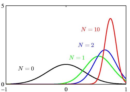
The above figure illustrates the Bayesian inference for the mean of a Gaussian distribution, for which the variance is assumed to be known. The curves show the prior distribution over 'mu' (the curve labeled N=0), which in this case is itself Gaussian, along with the posterior distributions for increasing number N of data points. The figure makes clear that as the number of data points increase, the posterior distribution peaks around the true value of the mean. This phenomenon is known as *Bayesian learning*.
For more information:


