Difference between revisions of "CBR logistic regression" - Rhea

Revision as of 00:24, 14 May 2014

Logistic regression

A slecture by ECE student Borui Chen

Partly based on the ECE662 Spring 2014 lecture material of Prof. Mireille Boutin.

Introduction

In the field of machine learning, one major topic is classification problem. Linear classifier is a class of algorithms that make the classification decision on a new test data point base on a linear combination of the features.

There are mainly two classes of linear classifier: Generative model and Discriminative model:

The generative model measures the joint distribution of the data and class.
- Examples are Naive Bayes Classifier, Linear Discriminant Analysis.

The discriminivative model makes no assumption on the joint distribution of the data. Instead, it takes the data as given and tries to maximize the conditional density (Prob(class|data)) directly.
- Examples are Logistic Regression, Perceptron and Support Vector Machine.

Intuition and derivation of Logistic Regression

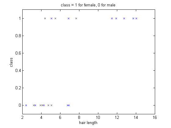
Consider a simple classification problem. The goal is to tell whether a person is male or female base on one feature: hair length. The data is given as $$ (x_i,y_i) $$ where i is the index number of the training set, and $$ x_i $$ is hair length in inches and $$ y_i=1 $$ indicates the person is male and 0 if female. Assume women has longer hair length the distribution of training data will look like this:

Clearly if a person's hair length is comparably long, being a female is more likely. If there is another person with hair length 10, we could say it's more likely to be a female. However, we don't have a description about how long is long enough to say a person is female. So we introduce the probability. We want to say that given a hair length is 10 inches, the probability of the person being a female is close to 1.

The intuition of logistic regression, in this example, is to assign a continuous probability to every possible value of hair length so that for longer hair length the probability of being a female is close to 1 and for shorter hair length the probability of being a female is close to 0. It is done by taking the linear combination of the feature and a constant and feeding it into a logistic function:

\begin{align} a_i &= \beta_0+\beta_1 x_i\\ &=\beta^T x_i \end{align}

L(a) = \frac{1}{1+e^{(-a)}}

Then the logistic function of $$ x_i $$ would be:

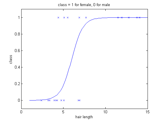
L(x_i) = Pr(Y_i=1|x_i) = Pr(female|x_i)= \frac{1}{1+e^{(-\beta^T x_i)}}

After some fitting optimization algorithm, the curve looks like the following:

Having this curve, we could develop an decision rule:

\text{This person is } \begin{cases} female, & \text{if }L(x_i)\ge 0.5\\ male, & \text{if }L(x_i) < 0.5 \end{cases}

More generally, the feature can be more than one dimension

$ x = (1,x_1,x_2,...,x_n)^T $

\beta = (\beta_0,\beta_1,\beta_2,...,\beta_n)^T

Note:

the decision boundary is linear:

\beta^T x_i = 0

For 1-D it's a point, 2-D it's a line and etc.

$\beta^T x_i$ is the log of the odd ratio:

\beta^T x_i = log\frac{Pr(female)}{Pr(male)}=log\frac{Pr(female)}{1-Pr(female)}

Having this setup, the goal is to find a $\beta$ to let the curve fit the data optimally. To solve the problem, it comes about Maximum Likelihood Estimation and Newton's method.

Maximum Likelihood Estimation

For the logistic regression, we need to figure out a best fit of the curve to the training data. To do this, we choose $\beta$ such that the likelihood of the joint distribution of the training data

$ Pr(Y_1=y_1,...,Y_n=y_n|x_1...x_n) $

is maximized.

From the likelihood function:

\begin{align} Pr(y|x) \triangleq Pr(Y_1=y_1,...,Y_n=y_n|x_1...x_n) &= \prod_{i=1}^n Pr(Y_i=y_i|x_i,\beta)\\ &= \prod_{i=1}^n Pr(Y_i=1|x_i,\beta)^{y_i} Pr(Y_i=0|x_i,\beta)^{1-y_i} \end{align}

For simple notation, let

\alpha = Pr(y_i=1|x_i,\beta)=\frac{1}{1+e^{-\beta^T x_i}}

Take the log of the likelihood function:

\begin{align} \log Pr(y|x) &= \sum_{i=1}^n y_i \log Pr(Y_i=1|x_i,\beta) + (1-y_i)\log Pr(Y_i=0|x_i,\beta)\\ &\triangleq \sum_{i=1}^n y_i \log \alpha + (1-y_i)\log (1-\alpha)\\ \end{align}

where

\begin{align} \alpha_i &= Pr(Y_i=1|x_i,\beta)=\frac{1}{1+e^{(-\beta^T x_i)}}\\ 1-\alpha_i &= Pr(Y_i=0|x_i,\beta)=\frac{1}{1+e^{(\beta^T x_i)}} \end{align}

and

\frac{\partial}{\partial\beta_j}\log \alpha_i = \frac{x_{ij}e^{-\beta^T x}}{1+e^{-\beta^T x}}=x_{ij}(1-\alpha)

\frac{\partial}{\partial\beta_j}\log (1-\alpha_i) = -x_{ij}+x_{ij}(1-\alpha)=-\alpha x_{ij}

Taking the derivative of the log likelihood with respect to $\beta$ :

\begin{align} \frac{\partial}{\partial\beta_j}\log Pr(y|x)&=\sum_{i=1}^n y_ix_{ij}(1-\alpha_i)+(1-y_i)x_{ij}\alpha_i\\ &= \sum_{i=1}^n (y_i - \alpha_i)x_{ij} \end{align}

If we set the above equation to zero, there is no close form solution, so we are going to use numerical optimization method to maximized the likelihood, namely, Newton's method.

Note

The goal is to maximize the above equation, however, in Newton's method it's easier to minimize the negative of the log likelihood function. In this case the derivatives becomes

\frac{\partial}{\partial\beta_j}\log Pr(y|x)=\sum_{i=1}^n (\alpha_i-y_i)x_{ij}

Numerical optimization - Newton's method

To apply the Newton's method, we need a gradient function of log likelihood with respect to $\beta$ , together with a Hessian matrix. from the last part, we've already computed the derivative for each $\beta_i$ , now we need to write it in matrix form.

\text{let }A= \begin{bmatrix} x_{11} & \cdots & x_{1d}\\ \vdots & \ddots & \vdots \\ x_{n1} & \cdots & x_{nd} \end{bmatrix}

where d is the dimension of the feature vector, n is size of training data set.

The gradient can be written as:

g(x,\beta) = \nabla \log Pr(y|x) = (\alpha-y)^T A

for the Hessian matrix, consider taking the derivative of the log likelihood function with respect to $\beta_j \text{ and }\beta_k$ .

\begin{align} \frac{\partial^2}{\partial\beta_j \partial\beta_k}\log Pr(y|x)&=\frac{\partial}{\partial\beta_k}\sum_{i=1}^n \alpha_ix_{ij}\\ &=\sum_{i=1}^n x_{ij}x_{ik}\alpha_i(1-\alpha_i)\\ &\triangleq z_j^T B z_k \end{align}

where $z_j = (x_{1j},\cdots,x_{nj})^T, B = diag(\alpha_1(1-\alpha_1),\cdots,\alpha_n(1-\alpha_n))$ . Then, can write Hessian matrix:

H(x,\beta) = \nabla^2 \log Pr(y|x) = A^TBA

With the equations of Gradient and Hessian matrix, we plug them into Newton's method iteration:

\beta_{k+1} = \beta_k - H^{-1}g

with some initialization $\beta_0$ .

Example

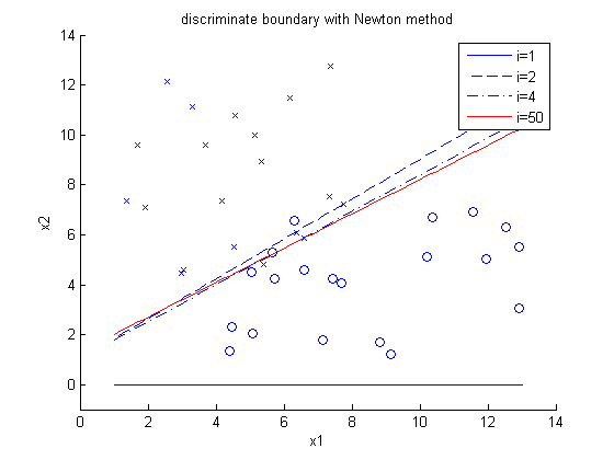
To show the performance of the implementation, 2-D uniform distributed training data is used. Following the implementation procedure described above, we get the following result:

In the plot, x and o represent two different classes.

Observations:

initial decision boundary is defined by equation

$ (0,0,1)(1,x_1,x_2)^T=0 $

The system converges fast, 4-th iteration is close enough to 50-th iteration.

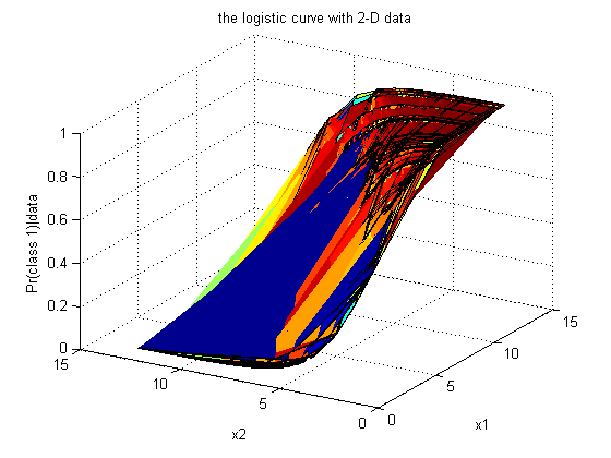
The following graph shows the logistic curve of the algorithm. It represents $$ Pr(class=1|data) $$

Summary

Logistic regression is an effective method that produces a linear classifier from labeled training data. Given a training data set, it tries estimate parameters $\beta$ in order to maximize the conditional log-likelihood function with a logistic probability model. then use Newton's method to find the best fit.

Reference

[1] Mireille Boutin, “ECE662: Statistical Pattern Recognition and Decision Making Processes,” Purdue University, Spring 2014
[2] http://www.stat.cmu.edu/~cshalizi/uADA/12/lectures/ch12.pdf
[3] Chong and Żak, An Introduction to Optimization, Fourth Edition, 2013

Questions and comments

If you have any questions, comments, etc. please post them on this page.

@@ Line 221: / Line 221: @@
 == Summary ==
-Logistic regression produces a linear classifier from labeled training data. Given a training data set, it tries to maximize the log-likelihood function with a logistic probability model, then use Newton's method to find the best fit of the parameters <math>\beta</math>.
+Logistic regression is an effective method that produces a linear classifier from labeled training data. Given a training data set, it tries estimate parameters <math>\beta</math> in order to maximize the conditional log-likelihood function with a logistic probability model. then use Newton's method to find the best fit.
 == Reference ==