Difference between revisions of "KnnDensityEstimation" - Rhea

Revision as of 13:39, 30 April 2014

K-Nearest Neighbors Density Estimation

A slecture by CIT student Raj Praveen Selvaraj

Completely based on the ECE662 Spring 2014 lecture material of Prof. Mireille Boutin.

Introduction

This slecture discusses about the K-Nearest Neighbors(k-NN) approach to estimate the density of a given distribution. The approach of K-Nearest Neighbors is very popular in signal and image processing for clustering and classification of patterns. It is an non-parametric density estimation technique which lets the region volume be a function of the training data. We will discuss the basic principle behind the k-NN approach to estimate density at any point x₀ and then move on to building a classifier using the k-NN Density estimate.

For a background knowledge on Local Density estimation methods, check the slecture on Introduction to local density estimation methods

K-Nearest Neighbor Density Estimation

The general formulation for density estimation states that, for N Observations x₁,x₂,x₃,...,x_n the density at a point x₀ can be approximated by,

\rho(x_{0}) = \frac{K}{NV}

where V is the volume of some neighborhood around x₀ and k denotes the number of observations that are contained within the neighborhood. The basic idea of k-NN is to extend the neighborhood, until the k nearest values are included where k ≥ 2. If we consider the neighborhood around x₀ as a sphere, the volume of the sphere is given by,

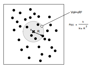
v_{k}(x_{0}) = \underset{h}{min}\left \{ \frac{\pi ^{n/2}.h^{n}}{\Gamma (\frac{n}{2} + 1)} \right \}

where $\Gamma (n) = (n - 1)!$ There are K samples within the sphere(including the boundaries) of radius h.This is illustrated in the below figure.

Figure 1. k-NN Neighborhood around a given point x

If x_l is the k^th closest sample point to x₀ then,

h_{k} = \parallel x_{l} - x_{0}\parallel

v_{k}(x_{0}) = \frac{\pi ^{n/2}}{\Gamma (\frac{n}{2} + 1)} . h_{k}^{n}

We approximate the density ρ(x₀) by,

\bar{\rho_{k}}(x_{0}) = \frac{k - \#s }{N.V_{k}(x_{0})}

where #s is the number of samples on the boundary of circle with radius h_k

Most of the time this estimate is,

\bar{\rho_{k}}(x_{0}) = \frac{k - 1 }{N.V_{k}(x_{0})}

The Estimated density at x₀ thorough K-NN gives the actual density at x₀

E(\bar{\rho_{k}}(x_{0})) = \rho(x_{0})

We will now prove the above claim that the estimated density is also the actual density at x₀

The above claim is true only in cases where the window function $\phi$ defines a region R with well defined boundaries.That is,

\phi(x) = \begin{Bmatrix}1 , x \ \epsilon \ R \\ 0, \ else \end{Bmatrix}

The random variable here is V_k(x₀)

Let,u be a small band along the boundary of R given by,

u = \int \rho(x)dx

Observation : $u \ \epsilon \ [0,1]$

Let G be the event that "K-1 samples fall inside " $$ R $$ and let H be the event that "1 sample falls inside the small band along the boundary"

Then,
$Prob(G, H) = Prob(G).Prob(H\mid G)$

$Prob(G) = \binom{N}{K-1}u^{k-1}(1-u)^{N-K+1}$

$Prob(H\mid G) = \binom{N-K+1}{1} \left ( \frac{\Delta u}{1-u} \right )\left ( 1 - \frac{\Delta u}{1-u} \right )^{N-K}$

where ${\Delta u}$ is given by,
${\Delta u} = \int \rho(x)dx$

$Prob(G,H) = \binom{N}{K-1} \binom{N-K+1}{1} \left ( \frac{\Delta u}{1-u} \right ) u^{K-1}\left ( 1 - \frac{\Delta u}{1-u} \right )^{N-K}(1-u)^{N-K+1}$

$Prob(G,H) = \frac{N!}{1!(N-K+1)!}.\frac{N-K+1}{1!(N-K)!}$

$Prob(G,H) = \frac{N!}{(k-1)!(N-K)!}.\Delta u(1 - u)^{N-K}u^{K-1}\left ( 1- \frac{\Delta u}{1-u}\right )^{N-K}$

$\left ( 1- \frac{\Delta u}{1-u}\right )^{N-K} = 1, when \ \Delta u \ is \ very \ small$

$Prob(G,H)\cong \Delta u. \frac{N!}{(k-1)!(N-K)!}.u^{k-1}(1-u)^{N-K}$

The Expected value of the density at x₀ by k-NN is given by,
$E(\bar{\rho }(x_{0})) = E(\frac{K-1}{N.V_{K}(x_{0})})$

recall that,

$u \cong \rho (x_{0}).V_{K}(x_{0})$

$\Rightarrow V_{K}(x_{0}) = \frac{u}{\rho (x_{0})}$

$E(\bar{\rho }(x_{0})) = E\left ( \frac{K-1}{N.u}.\rho (x_{0}) \right )$

$E(\bar{\rho }(x_{0})) = \frac{K-1}{N}\rho (x_{0}) E\left ( \frac{1}{u}\right)$

$E(\bar{\rho }(x_{0})) = \frac{K-1}{N}\rho (x_{0}) \int_{0}^{1}\frac{1}{u}\rho_{u}du$

$E(\bar{\rho }(x_{0})) = \frac{K-1}{N}\rho (x_{0}) \int_{0}^{1}\frac{1}{u}\frac{N!}{(K-1)!(N-K)!}u^{K-1}(1-u)^{N-K}du$

$E(\bar{\rho }(x_{0})) = \frac{K-1}{N}\rho (x_{0}) \int_{0}^{1}\frac{1}{u}\frac{N(N-1)!}{(K-1)(K-Z)!(N-K)!}u^{K-Z}(1-u)^{N-K}du$

$E(\bar{\rho }(x_{0})) = \frac{\rho (x_{0}).(N-1)!}{(K-Z)!}.\frac{1}{(N-K)!} \int_{0}^{1}u^{K-Z}(1-u)^{N-K}du$

Now, $\int_{0}^{1}u^{K-Z}(1-u)^{N-K}du = \frac{\Gamma (k-1)\Gamma (N-K+1)}{\Gamma (N)}$ and recall $\Gamma (n) = (n-1)!$ . Substituting these in the above equation we get,

$E(\bar{\rho }(x_{0})) = \rho(x_{0})$ as claimed.

How to classify data using k-NN Density Estimate

Having seen how the density at any given point x₀ is estimated based on the value of k and the given observations x₁,x₂,x₃,...,x_n, let's discuss about using the k-NN density estimate for classification. </br>

Method 1:

Let x₀ be a sample from Rⁿ to be classified.

Given are samples x_i1,x_x2,..,x_xn for i classes.

We now pick a "good" k_i for each class and a window function, and we try to approximate the density at x₀ for each class as discussed above.We then pick the class with the largest density at x₀ based on,

\rho(x_{0}\mid \omega _{i}) = \frac{k_{i} - 1 }{N_{i}.V_{k_{i}}(x_{0})}.Prob(\omega _{i})

If the priors of the classes are unknown, we use ROC curves to estimate the priors.
For more information on ROC curves check the slecture on ROC Curves

Method 2:

Given are samples x_i1,x_x2,..,x_xn from a Gaussian Mixture. We choose a good value for k and and a window function,

We then approximate the density at x₀ by,

\rho(x_{0}\mid \omega _{i}) = \frac{k_{i} - 1 }{N_{i}.V_{k_{i}}(x_{0})}

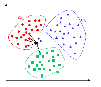
where V_i is the volume of the smallest window that contains k samples and k_i is the number of samples among these k that belongs to class i.

We pick a class i₀ such that,

Prob (\omega _{io}\mid x_{0})\geq Prob (\omega _{i}\mid x_{0}), \forall \ i = 1,2,..,c

On applying Bayes Rule, the above equation becomes,

\Rightarrow \rho(x_{0}\mid \omega _{i0}).Prob (\omega _{io})\geq \rho(x_{0}\mid \omega _{i}).Prob (\omega _{i}), \forall \ i = 1,2,..,c

If we assume that the priors of the classes are equal then,

\Rightarrow \rho(x_{0}, \omega _{i0}) \geq \rho(x_{0},\omega _{i}), \forall \ i = 1,2,..,c

Since the density is based on the number of neighbors of each class we can rewrite the above equation as,

k_{i0} \geq k_{i}, \forall \ i = 1,2,...,c

So classification using this method can also be thought of as assigning a class based on the majority vote of the k-Nearest Neighbors at any point x₀

Figure 2. Classifying a sample based on the majority vote of its neighbors

Conclusion

K-NN is a simple and intuitive algorithm that can be applied to any kind of distribution. It gives a very good classification rate when the number of samples is large enough. But choosing the best "k" for the classifier may be difficult. The time and space complexity of the algorithm is very high, and we need to make several optimizations for efficiently running the algorithm.

Neverthless, it's one among the most popular techniques used for classification.

References

[1] Mireille Boutin, "ECE662: Statistical Pattern Recognition and Decision Making Processes," Purdue University, Spring 2014.
[2] http://www.csd.uwo.ca/~olga/Courses/CS434a_541a/Lecture6.pdf
[3] http://research.cs.tamu.edu/prism/lectures/pr/pr_l8.pdf

If you have any questions, comments, etc. please post them on this page.

Back to ECE662, Spring 2014

@@ Line 149: / Line 149: @@
 If we assume that the priors of the classes are equal then,
 <center><math>\Rightarrow \rho(x_{0}, \omega _{i0}) \geq \rho(x_{0},\omega _{i}), \forall \ i = 1,2,..,c</math></center>
+Since the density is based on the number of neighbors of each class we can rewrite the above equation as,<br/>
 <center><math>k_{i0} \geq k_{i}, \forall \ i = 1,2,...,c</math></center>