| Line 1: | Line 1: | ||
| + | [[Category:2010 Spring ECE 662 mboutin]] | ||
| + | |||
| + | =Details of Lecture 8, [[ECE662]] Spring 2010= | ||
| + | |||
| + | |||
Classic central limit Thm (Second Fundamental probabilistic): | Classic central limit Thm (Second Fundamental probabilistic): | ||
| Line 73: | Line 78: | ||
--[[User:Gmoayeri|Gmoayeri]] 19:49, 9 May 2010 (UTC) | --[[User:Gmoayeri|Gmoayeri]] 19:49, 9 May 2010 (UTC) | ||
| + | |||
| + | Next: [[Lecture9ECE662S10|Lecture 9]] | ||
| + | ---- | ||
| + | [[OutlineECE662S10|Back to course outline]] | ||
| + | |||
| + | [[ 2010 Spring ECE 662 mboutin|Back to 2010 Spring ECE 662 mboutin]] | ||
| + | |||
| + | [[ECE662|Back to ECE662]] | ||
Revision as of 14:54, 9 May 2010
Details of Lecture 8, ECE662 Spring 2010
Classic central limit Thm (Second Fundamental probabilistic):
"The distribution of the average of a large number of samples from a distribution tends to be normal"
let X1,X2,...,Xn be n independent and identically distributed variables (i.i.d) with finite mean $ \mu $ and finite variance $ \sigma^2>0 $.Then as n increases the distribution of $ \Sigma_{i=1}^n \frac{X_i} {n} $ approaches $ N(\mu,\frac {\sigma^2}{n}) $.
More precisely the random variable $ Z_n = \frac{\Sigma_{i=1}^n X_i - n \mu}{\sigma \sqrt{n}} $ has $ P(Z_n)\longrightarrow N(0,1) $ when $ n \longrightarrow \infty $
More generalization of central limit Thm.
let X1,X2,...,Xn be n independent variables
Xi has mean $ \mu_i $ and finite variance $ \sigma^2 > 0 $ ,i=1,2,...,n
Then $ Z_n = \frac{\Sigma_{i=1}^n X_i - \Sigma_{i=1}^n \mu_i} {\sqrt{\Sigma_{i=1}^n \sigma^2}} $ has $ P(Z_n)\longrightarrow N(\mu ,\Sigma) $ when $ n \longrightarrow \infty $
Error bounds for Bayes decision rule:
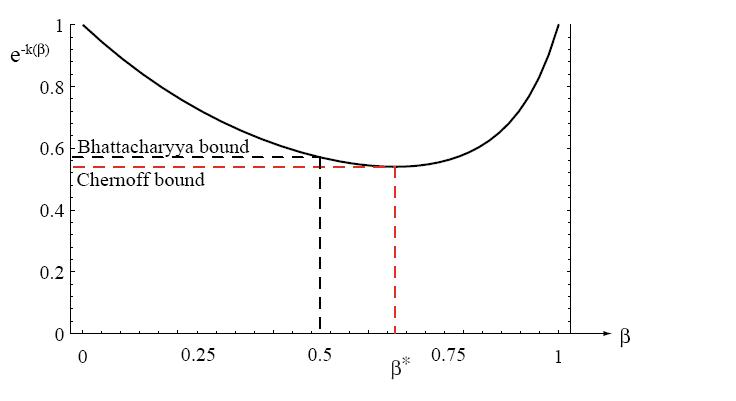
As we know Bayes decision rule guarantees the lowest average error rate; It Does not tell what the probability of error actually is. Therefore people try to find upper bounds for that: Chernoff and Bhattacharyya bounds
$ P(error)=\int_{R^n} p(error,x)dx = \int_{R^n} p(error|x)p(x)dx $
in two class case we have:
$ p(error|x) = min \{ p(\omega_1|x) , p(\omega_2|x) \} $ $ \Rightarrow P(error)= \int_{R^n}min\{p(\omega_1|x),p(\omega_2|x)\} p(x)dx $
as we know from Lemma: $ min \{a,b\}\leq a^\beta b^ {1-\beta} $, $ \forall a,b \geq 0 , \forall \beta s.t 0 \leq\beta\leq 1 $
$ P(error)\leq \int_{R^n} p(\omega_1 |x)^\beta p(\omega_2 |x)^{1-\beta} p(x) dx $ , $ \forall 0 \leq \beta \leq 1 $
$ P(error)\leq \int_{R^n} ({\frac {p(x|\omega)P(\omega_1)}{p(x)}})^\beta ({\frac {p(x|\omega_2)P(\omega_2)}{p(x)}})^{1-\beta} p(x) dx $ , $ \forall 0 \leq \beta \leq 1 $
$ P(error)\leq P(\omega_1) ^\beta P(\omega_2)^ https://kiwi.ecn.purdue.edu/rhea/skins/common/images/button_math.png{1-\beta} \int_{R^n} p(x|\omega_1)^\beta p(x|\omega_2)^{1-\beta} dx =: \varepsilon_\beta $ , $ \forall 0 \leq \beta \leq 1 $
The lower bound $ S:= min\varepsilon_\beta $ , $ \beta \in [0,1] $is an upper bound for P(error).
S is called "Chernoff Bound" and $ \varepsilon_{1/2} $ is called "Bhattacharyya Bound"
$ \varepsilon_{1/2}= \sqrt{P(\omega_1)P(\omega_2)} \int_{R^n} \sqrt{p(x|\omega_1)p(x|\omega_2)} dx = e^{-f(1/2)} \sqrt {P(\omega_1)P(\omega_2)} $
$ \varepsilon_\beta = P(\omega_1) ^\beta P(\omega_2)^ {1-\beta} \int_{R^n} p(x|\omega_1)^\beta p(x|\omega_2)^{1-\beta} dx = e^{-f(\beta)} P(\omega_1)^\beta P(\omega_2)^ {1-\beta} $
Here $ f(1/2) $ is "Bhattacharyya distance" and $ f(\beta) $ is "Chernof distance"
Especial case: Bounds for Gaussian density:
$ f(\beta)= {\frac{ \beta (1- \beta)}{2}} {(\mu_2 - \mu_1)^T} [ \beta \Sigma_1 + (1- \beta) \Sigma_2]^{-1} (\mu_2-\mu_1) + \frac {1}{2} ln{\frac {|\beta \Sigma_1 + (1-\beta) \Sigma_2|}{|\Sigma_1|^\beta |\Sigma_2|^ {1-\beta}}} $
$ f(1/2)=\frac{1}{8} (\mu_2 - \mu_1)^T [\frac {\Sigma_1 + \Sigma_2} {2}]^{-1} (\mu_2 - \mu_1) + \frac {1} {2} ln \frac {[\frac {\Sigma_1 + \Sigma_2} {2}]} {\sqrt {|\Sigma_1| |\Sigma_2|}} $
The Chernoff bound is found by analytically or numerically minimizing $ e^{-f(\beta)} $, therefore optimization is now in the one dimensional β space.

- Now consider a special case where : $ \Sigma_1 = \Sigma_2 =: \Sigma $
$ f(\beta) = \beta (1-\beta){(\mu_2 - \mu_1)^T} \Sigma^{-1}(\mu_2 - \mu_1) $
$ \frac {df(\beta)}{d\beta} = \frac {1-2\beta}{2}{(\mu_2 - \mu_1)^T} \Sigma^{-1}(\mu_2 - \mu_1)= 0 $
$ \Leftrightarrow \beta = \frac {1}{2} $ therefore Bhattacharyya Bound is optimum in this case.
- A closer look at f(1/2):
$ f(1/2)=\frac{1}{8} (\mu_2 - \mu_1)^T [\frac {\Sigma_1 + \Sigma_2} {2}]^{-1} (\mu_2 - \mu_1) + \frac {1} {2} ln \frac {[\frac {\Sigma_1 + \Sigma_2} {2}]} {\sqrt {|\Sigma_1| |\Sigma_2|}} $
As we see first term of this equation would be zero when $ \mu_1 = \mu_2 $; which shows class separability due to distance between means.(error would be higher when means of our classes are close to each other)
Second term of this equation would be zero when $ \Sigma_1 = \Sigma_2 $; which shows class separability due to difference of covariance matrices.
--Gmoayeri 19:49, 9 May 2010 (UTC)
Next: Lecture 9

