| (One intermediate revision by the same user not shown) | |||
| Line 9: | Line 9: | ||
</font size> | </font size> | ||
| − | A [ | + | A [http://www.projectrhea.org/learning/slectures.php slecture] by [[ECE]] student Chuohao Tang |
Partly based on the [[2014_Spring_ECE_662_Boutin_Statistical_Pattern_recognition_slectures|ECE662 Spring 2014 lecture]] material of [[user:mboutin|Prof. Mireille Boutin]]. | Partly based on the [[2014_Spring_ECE_662_Boutin_Statistical_Pattern_recognition_slectures|ECE662 Spring 2014 lecture]] material of [[user:mboutin|Prof. Mireille Boutin]]. | ||
Latest revision as of 09:47, 22 January 2015
Bayes rule in practice: definition and parameter estimation
A slecture by ECE student Chuohao Tang
Partly based on the ECE662 Spring 2014 lecture material of Prof. Mireille Boutin.
Content:
- Bayes rule for Gaussian data
- Procedure
- Parameter estimation
- Examples
- Summary
The purpose of this slecture is to establish a Bayes classifier system and how to apply it in practice. We assume the data are Gaussian distributed, and use maximum likelihood estimation to estimate the mean and variance of the training data. Then calculate the Bayesian probability and make the decision. We give 1d and 2d examples to illustrate how to apply the classifier.
1 Bayes rule for Gaussian data
Assume we have two classes $ \omega_1, \omega_2 $, and we want to classify the D-dimensional data $ \left\{{\mathbf{x}}\right\} $ into these two classes. To do so, we investigate the posterior probabilities of the two classes given the data, which are given by $ p(\omega_i|\mathbf{x}) $, where $ i=1,2 $ for a two-class classification. Using Bayes' theorem, these probabilities can be expressed in the form
where $ P(\omega_i) $ is the prior probability for class $ \omega_i $.
We will classify the data to $ \omega_1 $ if
and vise versa. Here $ g({\mathbf{x}}) $ is the discriminant function.
For a D-dimensional vector $ \mathbf{x} $, the multivariate Gaussian distribution takes the form
where $ \mathbf{\mu} $ is a D-dimensional mean vector, $ \mathbf{\Sigma} $ is a D×D covariance matrix, and $ |\mathbf{\Sigma}| $ denotes the determinant of $ \mathbf{\Sigma} $.
Then the discriminant function will be
So if $ g({\mathbf{x}})\geq 0 $, decide $ \omega_1 $; If $ g({\mathbf{x}}) < 0 $, decide $ \omega_2 $.
For k-classes classification problem, we decide the data belongs to $ c\omega_i $, where $ i=1,...,k $ if
2 Procedure
- Obtain training and testing data
We divide the sample data into training set and testing set. Training data is used to estimate the model parameters, and testing data is used to evaluate the accuracy of the classifier.
- Fit a Gaussian model to each class
- Parameter estimation for mean,variance
- Estimate class priors
We will discuss details to estimate these parameters in the following section.
- Calculate and decide
After obtaining the estimated parameters, we can calculate and decide which class a testing sample belongs to using Bayes rule.
$ \begin{align}if \ p({\mathbf{x}}|\omega_1)P(\omega_1)>p({\mathbf{x}}|\omega_2)P(\omega_2)\ decide\ \omega_1\\ if \ p({\mathbf{x}}|\omega_1)P(\omega_1)<p({\mathbf{x}}|\omega_2)P(\omega_2)\ decide\ \omega_2 \end{align} $
3 Parameter estimation
Given a data set $ \mathbf{X}=(\mathbf{x}_1,...,\mathbf{x}_N)^T $ in which the observations $ \{{\mathbf{x}_n}\} $ are assumed to be drawn independently from a multivariate Gaussian distribution (D dimension), we can estimate the parameters of the distribution by maximum likelihood. The log likelihood function is given by
By simple rearrangement, we see that the likelihood function depends on the data set only through the two quantities
These are the sufficient statistics for the Gaussian distribution. The derivative of the log likelihood with respect to $ \mathbf{\mu} $ is
and setting this derivative to zero, we obtain the solution for the maximum likelihood estimate of the mean
Use similar method by setting the derivative of the log likelihood with respect to $ \mathbf{\Sigma} $ to zero, we obtain and setting this derivative to zero, we obtain the solution for the maximum likelihood estimate of the mean
To estimate the class priors, we will count how much data are there for each class, so
4 Example
- 1-D case
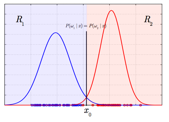
We draw samples from the following distributions. We divide the regions into $ R_1, R_2 $ according to the line $ P(\omega_1|x)=P(\omega_2|x) $, which will result in the minimum theoretical error. So we will decide $ \omega_1 $ if the sample falls into region $ R_1 $, and decide $ \omega_2 $ if the sample falls into region $ R_2 $.
- 2-D case
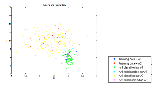
Suppose we have 200 2D training samples and 200 testing data. The parameters of the Gaussian distribution from which we drawn samples are
$ \begin{align} P({\mathbf{\omega}}_1)=0.4&, P({\mathbf{\omega}}_2)=0.6\\ {\mathbf{\mu}}_1=[6.0\ \ 16.0]^T &, {\mathbf{\mu}}_2=[5.4\ \ 20.0]^T\\ {\mathbf{\Sigma}}_1=\left[\begin{array}{lcr} 0.1 & 0\\ 0 & 1.0 \end{array}\right]&,{\mathbf{\Sigma}}_2=\left[\begin{array}{lcr} 0.5 & 0\\ 0 & 2.0 \end{array}\right] \end{align} $
Using training data, we obtain the estimated parameters as follows:
$ \begin{align} P_{est}({\mathbf{\omega}}_1)=0.44&, P_{est}({\mathbf{\omega}}_2)=0.55\\ {\mathbf{\mu}}_{1ML}=[6.1\ \ 16.0]^T &, {\mathbf{\mu}}_{2ML}=[5.4\ \ 19.8]^T\\ {\mathbf{\Sigma}}_{1ML}=\left[\begin{array}{lcr} 0.009 & 0.011\\ 0.011 & 0.84 \end{array}\right]&,{\mathbf{\Sigma}}_{2ML}=\left[\begin{array}{lcr} 0.2 & 0.042\\ 0.042 & 3.1 \end{array}\right] \end{align} $
The error rates are:
$ \begin{align} error\ rate (\omega_1 \ misclassified\ as\ \omega_2)=4.05%\\ error\ rate (\omega_2 \ misclassified\ as\ \omega_1)=3.97% \end{align} $
5 Summary
We establish a Bayes classifier system and how to apply it in practice. First we divide the samples into training data and testing data. We assume the data are Gaussian distributed, and use maximum likelihood estimation to estimate the mean and (co)variance of the training data. For testing data, then calculate the Bayesian probability and make the decision. We have 1d and 2d examples to illustrate how the classifier works.
Questions and comments
If you have any questions, comments, etc. please post them on this page.


