| (4 intermediate revisions by 2 users not shown) | |||
| Line 9: | Line 9: | ||
</font size> | </font size> | ||
| − | A [ | + | A [http://www.projectrhea.org/learning/slectures.php slecture] by [[ECE]] student Abdullah Alshaibani |
| − | Partly based on the [[ | + | Partly based on the [[2014_Spring_ECE_662_Boutin_Statistical_Pattern_recognition_slectures|ECE662 Spring 2014 lecture]] material of [[user:mboutin|Prof. Mireille Boutin]]. |
</center> | </center> | ||
---- | ---- | ||
| Line 284: | Line 284: | ||
In the figure above the circle represents R and the numbers represent the training points that fall inside R, each number represents a class. The class with the highest number of points inside R is the assigned class of <math>x_0</math>, which in this example is class 3. | In the figure above the circle represents R and the numbers represent the training points that fall inside R, each number represents a class. The class with the highest number of points inside R is the assigned class of <math>x_0</math>, which in this example is class 3. | ||
| + | ---- | ||
| + | |||
| + | == References == | ||
| + | [1] R.O. Duda, P.E. Hart, and D.G. Stork: Pattern Classification, Wiley, New York, NY, 2001 | ||
| + | [2] Mireille Boutin, ECE662: Statistical Pattern Recognition and Decision Making Processes, Purdue University, Spring 2014 | ||
---- | ---- | ||
---- | ---- | ||
---- | ---- | ||
| − | ==[[ | + | ==[[Parzen_Windows_slecture_review|Questions and comments]]== |
If you have any questions, comments, etc. please post them on [[Parzen_Windows_slecture_review|this page]]. | If you have any questions, comments, etc. please post them on [[Parzen_Windows_slecture_review|this page]]. | ||
---- | ---- | ||
[[2014_Spring_ECE_662_Boutin|Back to ECE662, Spring 2014]] | [[2014_Spring_ECE_662_Boutin|Back to ECE662, Spring 2014]] | ||
Latest revision as of 09:54, 22 January 2015
Parzen Windows
A slecture by ECE student Abdullah Alshaibani
Partly based on the ECE662 Spring 2014 lecture material of Prof. Mireille Boutin.
Contents
Introduction
As a Local Density Estimation method, Parzen Windows, focuses on estimating the density in a small region and making a decision based on that specific region. The density estimation relies on the specific test point being classified and the region around it. The reasoning behind it is to not focus on the accuracy of density estimation, but on the accuracy of decision making.
The idea is to create a smaller region, with the test point at its center, within the full region of the training data, and estimate the density in that small region and classify that test point based on the class with the highest density.
The method relies on the type or shape of the window used to form the smaller region.
Parzen Windows Method with a Cube Window
As mentioned before the reasoning behind it is to accurately make decisions and classify data. Thus the ideal method to explain how it works is to start with the classification process.
Given a set of training data in a region $ \Re^n $, and a point $ x_0 $ in the region $ \Re^n $.
a unit cube region $ R $ is created around $ x_0 $
using the following window function to count the samples in $ R $.
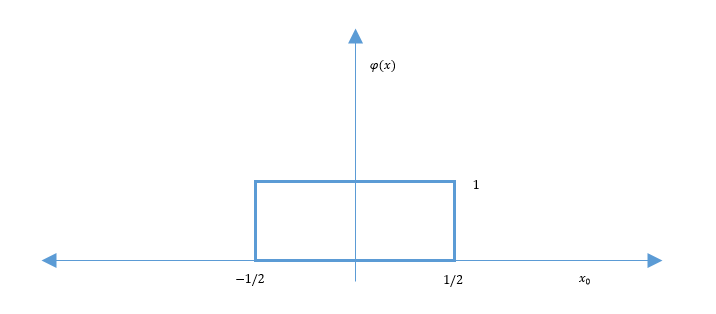
$ \phi(x) = \rho(x_1,x_2,...,x_n) = \begin{cases} 1 \quad if \left\vert x_1 \right\vert < \frac{1}{2}, \left\vert x_2 \right\vert < \frac{1}{2},..., \left\vert x_n \right\vert < \frac{1}{2} \\ 0 \quad else \\ \end{cases} $
Which yields the figure bellow.
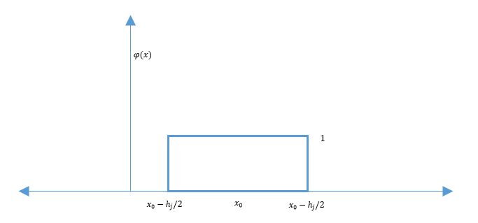
As we can see in the figure above, the window is not centered the point. To fix that issue we simply shift the window to be centered at $ x_0 $. Doing that would allow us to count the training data around the mean $ x_0 $.
$ \phi(x - x_0) = \begin{cases} 1 \quad if x \in R \\ 0 \quad else \\ \end{cases} $
So the number of training points inside $ R $ is defined by:
$ R = \sum_{l=1}^N \phi(x_l - x_0) $
$ \Rightarrow \widehat{\rho}(x_0) = \frac{1}{N} \frac{\sum_{l=1}^N \phi(x_l - x_0)}{\int_{\Re^n} \phi(x)\, dx} $
$ \Rightarrow \widehat{\rho_i}(x_0) = \frac{K_j}{j V_j} = \frac{1}{j V_j} \sum_{l=1}^j \phi(\frac{x_l - x_0}{h_j}) $
$ K_j = $ The number of training points in $ \{x_1,x_2,...,x_j\} $ inside $ R_j $
$ R_j = $ The region defined by $ \phi(\frac{x_l - x_0}{h_j}) $
$ V_j = $ The volume of $ R_j $
$ V_j = \int_{\Re^n} \phi(\frac{x}{h_j})\, dx $
Thus leading to:
After shifting the window it is now centered at $ x_0 $ and the $ \rho_i(x_0) $ would be the density estimate in that region for the class i. After applying the $ \rho_i(x_0) $ function on all the classes, we choose the class with the highest number density for $ x_0 $.
We can think of
$ \frac{1}{V_j} \phi(\frac{x_l - x_0}{h_j}) = \delta_j(x_j - x_0) \longrightarrow \delta(x - x_0) $
As an approximation of a unit impulse centered at $ x_0 $
$ \delta(x) = \begin{cases} \infty \quad if x = 0 \\ 0 \quad else \\ \end{cases} $
$ \int \delta(x)\, dx = 1 $
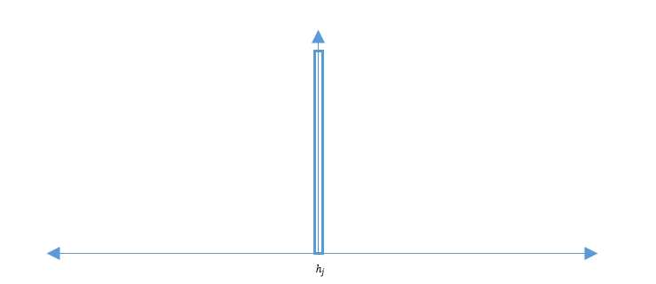
So as $ h_j \rightarrow 0 $ it will look like:
So the smaller $ h_j $ get the lower the number of training point that fall inside the window.
The Parzen Windows Method in General
We can pick any function $ \phi: \Re^n \rightarrow \Re \geqslant 0 $
such that
$ \lim_{h_j \to 0}\frac{1}{\int_{\Re^n} \phi(\frac{x}{h_j})\, dx} \phi\left (\frac{x}{h_j})\rightarrow \delta(x)\right ) $
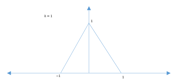 $ \phi(x) = \begin{cases} 1 - x \quad if 0 \leqslant x \leqslant 1 \\ 1 + x \quad if -1 \leqslant x \leqslant 0 \\ 0 \qquad\quad else \end{cases} $
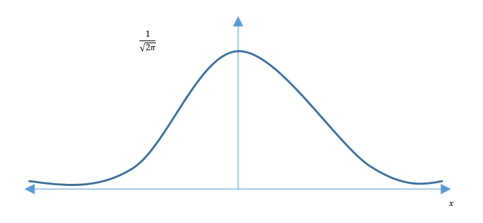 $ \phi(x) = \frac{1}{\sqrt{2 \pi}} e^{-\frac{x^2}{2}} $
$ \widehat{\rho}(x_0) = \frac{1}{N} \frac{1}{\int \phi(\frac{x_l - x_0}{h})\, dx} \sum_{l=1}^N \phi(\frac{x_l - x_0}{h}) $
Parameterized by h and the $ \phi $ function.
The main issues faced are:
- Bad estimates when no points exist in a region
- High computational cost
This works because instead of estimating
$ P = \int_{R} \rho(x)\, dx \rightarrow \rho(x_0) $
we now consider
$ P_\phi = \int_{\Re^n} \rho(x) \frac{\phi \left ( \frac{x - x_0}{h} \right )}{\int \phi(\frac{x}{h})\, dx}\, dx $
$ \quad = \rho(x) * \frac{\phi(\frac{x}{h})}{Vol(\phi)} \bigg|_{x = x_0} \xrightarrow[h \rightarrow 0]{} \rho(x) * \delta(x)\bigg|_{x = x_0} = \rho(x) $
Assuming $ \rho(x), \phi(x) $ continuous mean $ x_0 $.
Look at the convergence of $ \widehat{\rho_j}(x_0) $ in "mean square", i.e.
$ \lim_{j \to \infty} E(\widehat{\rho_j}(x_0)) = \rho(x_0) $
and
$ \lim_{j \to \infty} Var(\widehat{\rho_j}(x_0)) = 0 $
we have
$ \widehat{\rho_j}(x_0) = \frac{1}{j V_j} \phi(\frac{x_l - x_0}{h_j}), where V_j = \int \phi \left ( \frac{x}{h_j} \right ) \, dx $
$ \implies E(\widehat{\rho_j}(x_0)) = \frac{1}{j} \sum_{l=1}^j E(\frac{1}{V_j} \phi \left (\frac{x_l - x_0}{h_j} \right ) ) $
$ = \frac{1}{j} \sum_{l=1}^j \int \frac{1}{V_j} \phi \left (\frac{x_l - x_0}{h_j} \right ) \rho(x_l)\, dx_l $
$ = \frac{1}{j} j \int \frac{1}{V_j} \phi \left(\frac{x - x_0}{h_j}\right ) \rho(x)\, dx $
$ = \int \frac{1}{V_j} \phi \left(\frac{-1}{h_j} (x_0 - x)\right ) \rho(x)\, dx $
$ = \frac{1}{V_j} \phi \left(\frac{-x}{h_j} (x_0 - x)\right ) \rho(x) \bigg|_{x_0} \xrightarrow[h_j \to 0]{} \delta(-x) * \rho(x) \bigg|_{x_0} $
$ \delta(x) * \rho(x) \bigg|_{x_0} = \rho(x) $
Assuming $ \rho(x) and \phi(x) $ are continuous.
Important Observation
We do not need the number of samples → $ \infty $ to make
$ E(\widehat{\rho_j}(x_0)) \rightarrow \rho(x_0) $
we only need
- $ Vol(R_j) \xrightarrow[j \rightarrow \infty]{} 0 $
- or $ h_j \xrightarrow[j \rightarrow \infty]{} 0 $
There are a few setups that can be used to allow the use of Parzen Windows of which:
Setup 1
$ \mathfrak{D} \{x_1, x_2,...., x_N\} $ with N fixed
$ R_j \rightarrow \{x_0\} $
or $ \phi( \frac{x}{h_j}), with \quad h_j \to 0 $
with this setup $ E(\widehat{\rho_j}(x_0)) \xrightarrow[j \to \infty]{} \rho(x_0) $
Setup 2
$ \mathfrak{D} \{x_1, x_2,...., x_j\} $
$ R_j \rightarrow \{x_0\} $
or $ \phi( \frac{x}{h_j}), with \quad h_j \to 0 $
with this setup
$ E(\widehat{\rho_j}(x_0)) \xrightarrow[j \to \infty]{} \rho(x_0) \quad and \quad Var (\widehat{\rho_j}(x_0)) \rightarrow 0 $
for a carefully chosen $ R_j $ and $ h_j $
Now, how to make
$ Var(\widehat{\rho_j}(x_0)) \xrightarrow[j \to \infty]{} 0 $
$ Var(\widehat{\rho_j}(x_0)) = Var \left ( \sum_{l=1}^j \frac{1}{j V_j} \phi(\frac{x_l - x_0}{h_j}) \right ) $
$ = \sum_{l=1}^j Var \left ( \frac{1}{j V_j} \phi(\frac{x_l - x_0}{h_j}) \right ) $, by independence of $ x_l $'s
$ = j Var \left ( \frac{1}{j V_j} \phi(\frac{x - x_0}{h_j}) \right ) $
$ = E \left \{ \left ( \frac{1}{j V_j} \phi(\frac{x - x_0}{h_j}) - E(\frac{1}{j V_j} \phi(\frac{x - x_0}{h_j})) \right )^2 \right \} $
Recall $ E \left ( (x - E(x))^2 \right ) = E(x^2) - (E(x))^2 $
$ = j \left \{ E \left (\frac{1}{j^2} \frac{1}{V_j^2} \phi^2(\frac{x - x_0}{h_j}) \right ) - \left (E(\frac{1}{j V_j} \phi(\frac{x - x_0}{h_j})) \right )^2 \right \} $
$ \leqslant j E \left ( \frac{1}{j^2} \frac{1}{V_j^2} \phi^2(\frac{x - x_0}{h_j}) \right ) = \frac{1}{j} \int \frac{1}{V_j^2} \phi^2(\frac{x - x_0}{h_j}) \rho(x)\, dx $
$ = \frac{1}{j V_j} \int \frac{1}{V_j} \phi(\frac{x - x_0}{h_j}) \phi(\frac{x - x_0}{h_j}) \rho(x)\, dx $
$ \leqslant \frac{1}{j V_j} max \ \phi \int \frac{1}{V_j} \phi(\frac{x - x_0}{h_j}) \rho(x)\, dx $
$ = \frac{1}{j V_j} max\ \left ( \rho(x) * \frac{1}{V_j} \phi(\frac{-x}{h_j}) \right ) \Bigg|_{x_0} \leftarrow Convolution $
to make this converge to zero as $ j \to \infty $, we can
- Make $ V_j \to \infty $
- Which is not good since $ E(\widehat{\rho_j}(x_0)) \nrightarrow \rho(x_0) $
or
- Make $ j V_j \xrightarrow[j \to \infty]{} \infty $, and $ V_j \to 0 $
- e.g. $ V_j = \frac{1}{\sqrt{j}}, \quad V_j = \frac{7}{\sqrt{j}}, V_j = \frac{1000000}{\sqrt{j}} $, etc
- Make $ V_j $ constant so $ \frac{1}{j V_j} \to 0 $
- But then $ E(\widehat{\rho_j}(x_0)) \nrightarrow \rho(x_0) $
A Simple Way to Make Decisions using Parzen Windows
Given labeled samples $ \{x_1, x_2, x_3,..., x_N\} $ drawn from a mixture density
if we fix a point $ x_0 \in \Re^n $ and a region R around $ x_0 $
We have $ \rho(x_0, \omega_i) \equiv \frac{\# \ of \ points \ from \ class \ i \ (in \ \mathfrak{D}) \ in \ R}{N \ . \ Volume(R)} $
Instead of R we can choose to fix a window function $ \phi $
$ \rho(x_0, \omega_i) \equiv \frac{\sum_{l=1}^N \phi(\frac{x_l - x_0}{h})}{N \int \phi(\frac{x}{h})\, dx} $
$ x_l $ in class i
We pick the class $ \omega_{i0} $ such that
$ Prob(\omega_{i0} | x_0) \geqslant Prob(\omega_i | x_0) \quad \forall i = 1, 2,..., c $
By Bayes Theorem
$ \Leftrightarrow \rho(x_0 | \omega_{i0}) \geqslant \rho(x_0 | \omega_0) \quad \forall i = 1, 2,..., c $
$ \Leftrightarrow \underbrace{\frac{\sum_{l=1}^N \phi(\frac{x_l - x_0}{h})}{N \int \phi(\frac{x}{h})\, dx} }_{x_l \ in \ class \ \omega_{i0}} \geqslant \underbrace{\frac{\sum_{l=1}^N \phi(\frac{x_l - x_0}{h})}{N \int \phi(\frac{x}{h})\, dx} }_{x_l \ in \ class \ \omega_{i}} $
$ \Leftrightarrow \underbrace{\sum_{l=1}^N \phi(\frac{x_l - x_0}{h}) }_{x_l \ in \ class \ \omega_{i0}} \geqslant \underbrace{\sum_{l=1}^N \phi(\frac{x_l - x_0}{h})}_{x_l \ in \ class \ \omega_{i}} $
$ Or \ K_{io} \geqslant K_i $
where $ K_i $ is the number of points (in $ \mathfrak{D} $) from class i inside R.
Assign $ x_0 $ to the majority vote weighted of the neighbors inside R.
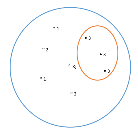
In the figure above the circle represents R and the numbers represent the training points that fall inside R, each number represents a class. The class with the highest number of points inside R is the assigned class of $ x_0 $, which in this example is class 3.
References
[1] R.O. Duda, P.E. Hart, and D.G. Stork: Pattern Classification, Wiley, New York, NY, 2001
[2] Mireille Boutin, ECE662: Statistical Pattern Recognition and Decision Making Processes, Purdue University, Spring 2014
Questions and comments
If you have any questions, comments, etc. please post them on this page.

