| (10 intermediate revisions by 4 users not shown) | |||
| Line 1: | Line 1: | ||
<br> | <br> | ||
<center><font size="4"></font> | <center><font size="4"></font> | ||
| − | <font size="4">'''Bayes rule in practice''' <br> </font> <font size="2">A [ | + | <font size="4">'''Bayes rule in practice''' <br> </font> <font size="2">A [http://www.projectrhea.org/learning/slectures.php slecture] by Lu Wang </font> |
| − | + | Partly based on the [[2014_Spring_ECE_662_Boutin_Statistical_Pattern_recognition_slectures|ECE662 Spring 2014 lecture]] material of [[user:mboutin|Prof. Mireille Boutin]]. | |
</center> | </center> | ||
---- | ---- | ||
| Line 9: | Line 9: | ||
---- | ---- | ||
| − | == 1. Bayes rule for Gaussian data == | + | == 1. Introduction == |
| + | |||
| + | This slecture demonstrates the general procedures of Bayes Classifier in two-class scenario under Gaussian assumption. We first derive the discriminant function according to Bayes rule. Then we introduce the density estimation methods in general followed by an example of the maximum likelihood estimation (MLE) of Gaussian data. Finally, Bayes classifier in practice is illustrated through an experiment where MLE is applied to the Gaussian training data with unknown parameters, and testing data is classified with Bayes rule.<br> | ||
| + | |||
| + | <br> | ||
| + | |||
| + | ---- | ||
| + | |||
| + | == 2. Bayes rule for Gaussian data == | ||
Given data x ∈ R<span class="texhtml"><sup>''d''</sup></span> and N categories {w<span class="texhtml"><sub>''i''</sub></span>}, i=1,2,…,N, we decide which category the data corresponds to by computing the probability of the N events. We’ll pick the category with the largest probability. Mathematically, this can be interpreted as: | Given data x ∈ R<span class="texhtml"><sup>''d''</sup></span> and N categories {w<span class="texhtml"><sub>''i''</sub></span>}, i=1,2,…,N, we decide which category the data corresponds to by computing the probability of the N events. We’ll pick the category with the largest probability. Mathematically, this can be interpreted as: | ||
| Line 36: | Line 44: | ||
\end{align} | \end{align} | ||
</math></center> | </math></center> | ||
| − | <br>For two-class case, generate the discriminant function as | + | <br>For the two-class case, generate the discriminant function as |
<center><math>g\left(x\right) = g_{1}\left(x\right) - g_{2}\left(x\right);</math><br></center> <center>decide w<sub>1</sub> if g(x) > 0;<br></center> <center>else decide w<sub>2</sub>.</center> | <center><math>g\left(x\right) = g_{1}\left(x\right) - g_{2}\left(x\right);</math><br></center> <center>decide w<sub>1</sub> if g(x) > 0;<br></center> <center>else decide w<sub>2</sub>.</center> | ||
---- | ---- | ||
| − | == | + | == 3. How to evaluate parameters for Gaussian data == |
If the parameters for Gaussian, μ<sub>i</sub> and Σ<sub>i</sub> are unknown for category w<sub>i</sub>, we then need to estimate the parameters based on the information of data samples. | If the parameters for Gaussian, μ<sub>i</sub> and Σ<sub>i</sub> are unknown for category w<sub>i</sub>, we then need to estimate the parameters based on the information of data samples. | ||
| − | ''' | + | '''3.1 Generate training and testing samples'''<br> Given the data samples with known category, we are able to estimate the parameters for the Gaussian distribution. Data samples are divided into training samples and testing samples, where μi and Σi are estimated from the training samples first, and then evaluated based on the testing samples. Generally, the more training samples, the more accurate the estimation will be. Also, it is important to select training samples that can represent the distribution of the population.<br> |
| − | ''' | + | '''3.2 How to estimate μi and Σi'''<br> There are various methods to estimate the density distribution. Generally speaking, we have parametric and non-parametric density estimation methods. <br> Parametric methods usually derive mathematical expression involving the training data for each parameter. Classic parametric methods include Maximum Likelihood estimation (MLE), and Bayesian Parametric estimation (BPE). However, parametric methods would result in large error rate if the density assumption (such as Gaussian in our case) is incorrect. <br> Non-parametric methods do not require the foreknowledge of the density distribution. In fact, they do not estimate the parameters; instead, they estimate the density for each point to be classified. Parzen window and K-nearest neighbors (KNN) are two of the famous non-parametric methods. Two common concerns about non-parametric methods are computational complexity and the number of training samples required.<br> |
| − | ''' | + | '''3.3 Estimate μ and Σ through MLE''' |
Let D = {x<sub>1</sub>,x<sub>2</sub>,...,x<sub>N</sub>} to be a set of iid samples from the Gaussian distribution with μ and Σ unknown. The MLE for μ and Σ are<br> | Let D = {x<sub>1</sub>,x<sub>2</sub>,...,x<sub>N</sub>} to be a set of iid samples from the Gaussian distribution with μ and Σ unknown. The MLE for μ and Σ are<br> | ||
| Line 58: | Line 66: | ||
---- | ---- | ||
| − | == | + | == 4. Example: data classification based on the Bayes rule == |
Assume a two-claess case, the total population for class 1 and class 2 are 10000, where the prior probability for class 1 is 0.3, so that the prior probability for class 2 is 0.7. The data of category 1 are distributed as N(1, 2), while those of category 2 are distributed as N(4, 1). | Assume a two-claess case, the total population for class 1 and class 2 are 10000, where the prior probability for class 1 is 0.3, so that the prior probability for class 2 is 0.7. The data of category 1 are distributed as N(1, 2), while those of category 2 are distributed as N(4, 1). | ||
| − | 200 training samples are randomly chosen from the population pool. In this sense, the proportion of class 1 in the training samples won't necessarily be the same as its proportion in the whole population. We then pick another 500 test samples from the population randomly. Keep in mind that we know the classification for each data point no matter for training samples or test samples. We build the discriminant function based on the classification of the training sample, while test the accuracy by compare the decisions made for the test sample and their ground truth. | + | 200 training samples are randomly chosen from the population pool. In this sense, the proportion of class 1 in the training samples won't necessarily be the same as its proportion in the whole population. We then pick another 500 test samples from the population randomly. Keep in mind that we know the classification for each data point no matter for training samples or test samples. We build the discriminant function based on the classification of the training sample, while test the accuracy by compare the decisions made for the test sample and their ground truth.<br> |
| + | |||
| + | The above procedures are repeated for 100 times. Figure 1 shows the estimated μi and Σi for each trail, the mean vaue, and the standard deviation. The estimation of the four parameters are all very close to the true value. The MLE of μ for Gaussian is unbiased, while the MLE of Σ is unbiased. | ||
| + | |||
| + | <br> | ||
| + | <center>[[Image:S1.png|thumb|left|750px]]</center> <center>Fig 1. Estimated μi and Σi for each trail</center> | ||
| + | <br> | ||
| + | |||
| + | <br> We now investigate the accuracy of classification. Plug each test sample into the discriminant function g(x) defined in Part 1, and decide which category this sample belongs to. We then compare the decision with the ground truth. Define error rate of the model as | ||
| + | <center><math>error\ rate = \frac{number\ of\ misclassified\ test\ samples}{number\ of\ test\ smaples}\times100\%</math>.<br></center> | ||
| + | Figure 2 illustrate the histogram of error rate for the 100 trails. | ||
| + | <center>[[Image:ErrorRate.jpg|thumb|left|750px]]</center> <center>Fig 2. Histogram of the error rate for 100 runs</center> | ||
| + | <br> | ||
| + | |||
| + | ---- | ||
| + | |||
| + | == [[Bayes rule in practice review|Questions and comments]] == | ||
| + | |||
| + | If you have any questions, comments, etc. please post them on [[Bayes rule in practice review|this page]]. | ||
| + | ---- | ||
| + | |||
| + | [[2014 Spring ECE 662 Boutin|Back to ECE662, Spring 2014]] | ||
| − | [[ | + | [[Category:Slecture]] [[Category:ECE662Spring2014Boutin]] [[Category:ECE]] [[Category:ECE662]] [[Category:Pattern_recognition]] |
Latest revision as of 09:47, 22 January 2015
Bayes rule in practice
A slecture by Lu Wang
Partly based on the ECE662 Spring 2014 lecture material of Prof. Mireille Boutin.
Contents
1. Introduction
This slecture demonstrates the general procedures of Bayes Classifier in two-class scenario under Gaussian assumption. We first derive the discriminant function according to Bayes rule. Then we introduce the density estimation methods in general followed by an example of the maximum likelihood estimation (MLE) of Gaussian data. Finally, Bayes classifier in practice is illustrated through an experiment where MLE is applied to the Gaussian training data with unknown parameters, and testing data is classified with Bayes rule.
2. Bayes rule for Gaussian data
Given data x ∈ Rd and N categories {wi}, i=1,2,…,N, we decide which category the data corresponds to by computing the probability of the N events. We’ll pick the category with the largest probability. Mathematically, this can be interpreted as:
According to Bayes rule:
In our case, the data is distributed as Gaussian. So we have,
Let
Now we have,
For the two-class case, generate the discriminant function as
3. How to evaluate parameters for Gaussian data
If the parameters for Gaussian, μi and Σi are unknown for category wi, we then need to estimate the parameters based on the information of data samples.
3.1 Generate training and testing samples
Given the data samples with known category, we are able to estimate the parameters for the Gaussian distribution. Data samples are divided into training samples and testing samples, where μi and Σi are estimated from the training samples first, and then evaluated based on the testing samples. Generally, the more training samples, the more accurate the estimation will be. Also, it is important to select training samples that can represent the distribution of the population.
3.2 How to estimate μi and Σi
There are various methods to estimate the density distribution. Generally speaking, we have parametric and non-parametric density estimation methods.
Parametric methods usually derive mathematical expression involving the training data for each parameter. Classic parametric methods include Maximum Likelihood estimation (MLE), and Bayesian Parametric estimation (BPE). However, parametric methods would result in large error rate if the density assumption (such as Gaussian in our case) is incorrect.
Non-parametric methods do not require the foreknowledge of the density distribution. In fact, they do not estimate the parameters; instead, they estimate the density for each point to be classified. Parzen window and K-nearest neighbors (KNN) are two of the famous non-parametric methods. Two common concerns about non-parametric methods are computational complexity and the number of training samples required.
3.3 Estimate μ and Σ through MLE
Let D = {x1,x2,...,xN} to be a set of iid samples from the Gaussian distribution with μ and Σ unknown. The MLE for μ and Σ are
See Tutorial on Maximum Likelihood Estimation: A Parametric Density Estimation Method for more details.
4. Example: data classification based on the Bayes rule
Assume a two-claess case, the total population for class 1 and class 2 are 10000, where the prior probability for class 1 is 0.3, so that the prior probability for class 2 is 0.7. The data of category 1 are distributed as N(1, 2), while those of category 2 are distributed as N(4, 1).
200 training samples are randomly chosen from the population pool. In this sense, the proportion of class 1 in the training samples won't necessarily be the same as its proportion in the whole population. We then pick another 500 test samples from the population randomly. Keep in mind that we know the classification for each data point no matter for training samples or test samples. We build the discriminant function based on the classification of the training sample, while test the accuracy by compare the decisions made for the test sample and their ground truth.
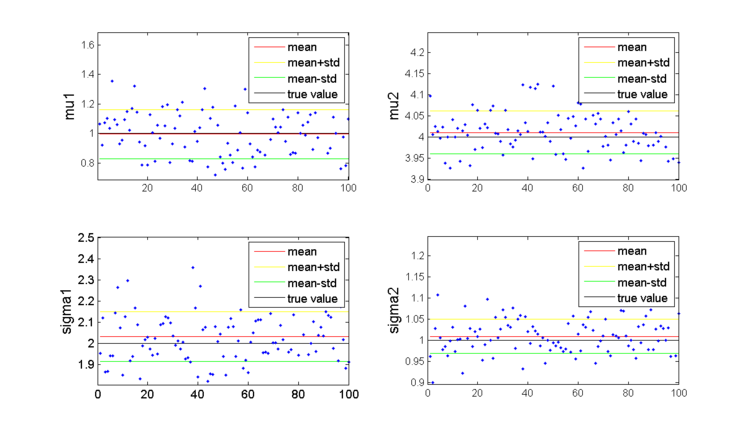
The above procedures are repeated for 100 times. Figure 1 shows the estimated μi and Σi for each trail, the mean vaue, and the standard deviation. The estimation of the four parameters are all very close to the true value. The MLE of μ for Gaussian is unbiased, while the MLE of Σ is unbiased.
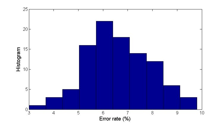
We now investigate the accuracy of classification. Plug each test sample into the discriminant function g(x) defined in Part 1, and decide which category this sample belongs to. We then compare the decision with the ground truth. Define error rate of the model as
Figure 2 illustrate the histogram of error rate for the 100 trails.
Questions and comments
If you have any questions, comments, etc. please post them on this page.


