Revision as of 06:31, 15 May 2014

PDF Version Available here: pdf

Introduction

Linear discriminant analysis is a technique that classifies two classes by drawing decision regions defined only by a hyperplane. This is a somewhat different strategy than what has been used elsewhere in this course. While other techniques for decision making first concerned themselves with estimating the probability distributions of the classes from training data, this technique instead just looks to find decent decision regions for the two classes that best fit the training data. For classification purposes, the side of the hyperplane that the data lies on determines which class the data belongs to.

Discriminant Functions

In statistical decision theory, the optimal Bayesian decision rule is given as the following in the two class case:

$ p(x|\theta_1) Prob(\theta_1) - p(x|\theta_0) Prob(\theta_0) \quad\mathop{\gtreqless}_{\theta_0}^{\theta_1} 0. $

Here θ_i refers to the classes, x refers to the data point to be classified, Prob(θ_i) is the prior probability of class i, and p(x | θ_i) is the probabilty distribution function for class i. If this expression is positive, then the data is decided to be of class 1. If the expression is negative, then the data is decided to be of class 0.

No matter the form of the decision rule, it could be restated as the following:

$ f(x) \quad\mathop{\gtreqless}_{\theta_0}^{\theta_1} 0. $

Here f is just some function. In particular, it is called a discriminant function. Finding where this function equals zero gives the hypersurface or hypersurfaces separating the classes. Some other function could be used as the discriminant function. In LDA, the function is taken to be

$ \vec{c} \cdot (1, \vec{x}) \quad\mathop{\gtreqless}_{\theta_0}^{\theta_1} b $

where $ (1, \vec{x}) $ is concatenating the sample vector with a one, pushing it up to a higher dimension, and $ \vec{c} $ and b remain to be found. This equation describes decision regions separated by a hyperplane. $ \vec{c} $ is a vector normal to the dividing hyperplane, and b effectively shifts the hyperplane from the origin and is sometimes called the margin. The following sections explain the reasoning behind the concatenation along with how to find $ \vec{c} $ and b under certain assumptions.

Set up and Tricks

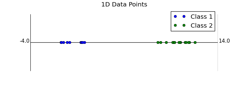
There are a number of tricks that are used in the set up for LDA. The first and most important is the concatenation trick. This trick takes a sample vector and pushes it up one dimension by adding a constant element to it. Why this is a good idea isn’t immediately clear, but looking at the effect of this choice starting in one dimension is very illustrative. In one dimension, the clustered data for two classes could look like the following.

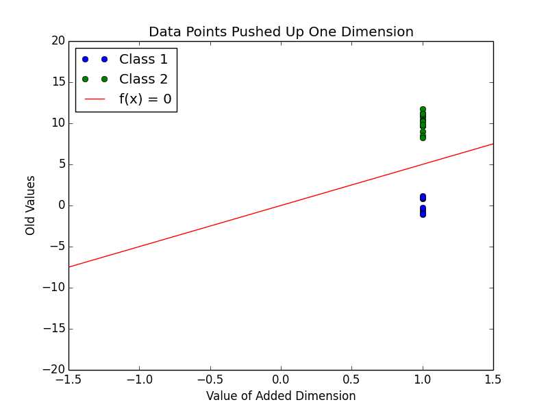
Now, the first trick is adding a dimension to this. Below is a plot of $ (1, \vec{x}) $.

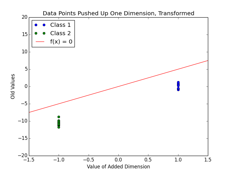
Also in this plot is a line showing where a proposed linear discriminant function is 0. The added dimension here allows this linear separation. Because this is only in two dimensions, the dividing hyperplane is only a line. This line is actually still to be determined; the line here is just meant to be used as an example. One way to define this line is using the vector $ \vec{c} $, which is set to be normal to the line. This gives rise to the form of the discriminant expression, $ \vec{c} \cdot (1, \vec{x}) \quad\mathop{\gtreqless}_{\theta_0}^{\theta_1} b $. Here, b is set to be 0, so that the dividing line goes through the origin. Still, in this case, it divides the data. One more trick can be used to find a “better” value for b. The below plot transforms the data so that all the class two data points are multiplied by -1.

This transformation makes it easier to look at one particular way to set b, which shifts $ \vec{c} $ around. As seen in class before for the other types of classifiers, usually this sort of translation is determined by the priors of the two class distributions. Most of the time for linear classifiers this sort of thought process isn’t used, though. Instead, b is picked by shifting $ \vec{c} $ from the origin so that it touches the closest point(s) from both classes. In other words, b is the shortest distance from the hyperplane to any of the data points. For this reason, b is sometimes called the margin.

A better, animated plot of this example can be found at https://www.projectrhea.org/rhea/index.php/Image:Lecture11-1_OldKiwi.gif from the 2008 Rhea notes for this course. Still, this leaves the choice of $ \vec{c} $. In the next section we will look at how to choose it under the regime prescribed by Fisher’s linear discriminant.

Fisher’s Linear Discriminant

Fisher’s linear discriminant chooses $ \vec{c} $ by setting a particular cost function $ J(\vec{c}) $ and solving for the $ \vec{c} $ that maximizes it. $ J(\vec{c}) $ is given by the following:

$ J(\vec{c}) = \frac{||m_1-m_2||^2_2}{s_1^2+s_2^2} $

where N_i is the number of training samples that belong to class i,

$ m_i = \frac{1}{N_i}\sum_{\vec{X_j} \in i} \vec{c} \cdot \vec{X_j}, $

and

$ s_i = \sum_{\vec{X_j} \in i} (\vec{c} \cdot \vec{X_j} - m_i)^2. $

The value of m_i can be taken to be the mean value of the projection of class i onto the normal vector. s_i is called the scatter of the data, and is similar to the idea of sample variance. Intuitively, this cost function is maximized when the projected means are far apart, and the scatters are small. This intuitive definition of the cost function can be reformulated to the following:

$ J(\vec{c}) = \frac{\vec{c}^T S_B \vec{c}}{\vec{c}^T S_W \vec{c}} $

where

$ S_B = (\hat{\vec{\mu_1}} - \hat{\vec{\mu_2}})(\hat{\vec{\mu_1}} - \hat{\vec{\mu_2}})^T $

and

$ S_W = \sum_{\vec{X_j} \in 1} (\vec{X_j} - \hat{\vec{\mu_1}})(\vec{X_j} - \hat{\vec{\mu_1}})^T + \sum_{\vec{X_j} \in 2} (\vec{X_j} - \hat{\vec{\mu_2}})(\vec{X_j} - \hat{\vec{\mu_2}})^T $

with $ \hat{\vec{\mu_i}} $ taken to be the sample mean of class i. Luckily, this can be maximized analytically using linear algebra. The result of that gives

$ \vec{c} = const \cdot S_W^{-1}(\hat{\vec{\mu_1}} - \hat{\vec{\mu_2}}). $

Notice that there are infinitely many valid choices of $ \vec{c} $, but they all point in the same direction. This makes sense since $ \vec{c} $ is meant to be a vector normal to the dividing hyperplane. The choice of the constant will affect the choice of margin b also, but simply by a multiplicative scalar.

It should now be noted that Fisher’s linear discriminant looks awfully like the result for the Bayesian decision rule with two Gaussians of differing means but identical covariances matrices. This makes sense, since in that particular set up, the resulting decision regions are always defined by a hyperplane. This would also mean that the value b that shifts around the hyperplane between the two clusters would be picked according to the priors of the two classes. When priors are equal, $ b = \vec{c} \cdot (\hat{\vec{\mu_1}} + \hat{\vec{\mu_2}}) / 2 $, which puts the hyperplane directly between the two class clusters.

It should also be noted that this technique works for non-linearly separated data. This is obviously critically important, since most data wont actually be linearly separable. Other choices of cost function can also be picked to handle this problem.

Final Notes

In this short slecture, linear discriminant analysis and Fisher’s linear discriminant were discussed. These linear classifier techniques are very useful for dimensionality reduction, and are also used in support vector machines. This technique has the advantage of making the classification of data points very fast, since it only depends on a dot product. Comparatively, other tests such as density estimation based tests could require much more complicated calculations or algorithms to classify data points. If the data is roughly linearly separable, the other techniques will be more expensive with little or no actual improvement in classification performance.

References

1. Mirielle Boutin, “Lectures Notes from ECE662: Statistical Pattern Recognition and Decision Making Processes.” Purdue University, Spring 2014.

2. “Fisher Linear Discriminant.” Rhea. Purdue University, n.d. Web. 02 May 2014. https://www.projectrhea.org/rhea/index.php/Fisher_Linear_Discriminant_OldKiwi.

Questions and comments

If you have any questions, comments, etc. please post them on this page.

Back to ECE662, Spring 2014