Revision as of 16:44, 30 April 2014

Introduction

K Nearest Neighbors is a classification algorithm based on local density estimation.

A classifier is given a set of $ N $ data-points (usually vectors) $ x_{1}, x_{2}, ..., x_{N} $ along with corresponding labels $ y_{1}, y_{2}, ..., y_{N} $ from some set of $ C $ classes $ w_1,w_2,...w_C $.

Together these are often called the training set, because they are used to "train" the classifier.

Given the training set, the goal of a classifier is to take a new data-point $ x_{0} $, and assign it a class label.

If the data-points from each class are random variables, then it can be proven that the optimal decision rule to classify a point $ x_0 $ is Bayes Rule, which is to choose the class for which $ P(w_i|x_0) $, the is highest.

Therefore, it is desirable to assume that the data-points are random variables, and attempt to estimate $ P(w_i|x_0) $, in order to use it to classify the points.

By Bayes Theorem,

$  P(w_i|x_0) = P(x_o|w_i)P(w_i) $.

This is advantageous because it is often easier to estimate $ P(x_o|w_i) $ and $ P(w_i) $ separately than to estimate $ P(w_i|x_0) $ directly.

K Nearest Neighbors

As a density estimator

This method belongs to the class of local density estimation methods because it forms a separate density estimate locally around each test point $ x_0 $. This is in contrast to non-local methods which assume a symbolic form (for example gaussian) for the distributions and estimate the entire distribution by finding the parameters (the mean and variance for the gaussian example) of that distribution.

K Nearest Neighbors is not usually used to estimate explicitly $ P(w_i|x_0) = P(x_o|w_i)P(w_i) $, but instead does so implicitly, and chooses the class with the highest estimated $ P(w_i|x_0) $.

The density $ P(x_0|w_i) $ at a point $ x_0 $ can be estimated by choosing a region $ R $ with volume $ V_R $ centered at $ x_0 $, and setting $ \hat{P}(x_0|w_i) $, the density estimate at $ x_0 $, to be $ \hat{P}(x_0|w_i) = \frac{k}{NV_R} $.

The intuition behind this estimate is that the expected value of the number of points $ k $ that fall within region $ R $ is proportional to the average probability density in the region, the number total number of points $ N $ drawn from the distribution, and to the volume $ V_R $ of the region. Therefore, one can estimate the average density in the region around $ x_0 $, and use it as the estimate at $ x_0 $.

The more points in the training set, the more likely the ratio of points in and out of the region will be close to the expected ratio, and the more likely the estimate is to be close to the true value of the average region density. However, no matter how many points are available, the estimate is an average over the region R, not the value of the density at point $ x_0 $.

However, there is a trade-off for choosing the size of R: On the one hand, it is desirable for the region to be very small, but on the other hand, the smaller it is, the fewer points will fall in the region. If R is too small, there will be too few (or possibly zero) points that fall into R, resulting in an inaccurate estimate. Additionally, if a fixed size R is used, it may over-average in some regions, yet still be too small to include enough points in other regions.

K Nearest neighbors' answer to this trade-off is to avoid choosing a region size, and instead choose the value of k. The region size is then determined for each point $ x_0 $ as the minimum (technically the infimum) volume $ V_k(x_0) $ needed to include k datapoints. This allows the region size to change dynamically according to the number of points near $ x_0 $.

It can be proved that $ E[\frac{k-k_b}{NV_k(x_0)}] = P(x_0|w_i) $ for all k>=2.

Where $ k_b $ is the number of points on the boundary of the region, which should not be counted.

It is not necessary to have a region with distinct boundaries, nor to weigh all points in the region equally. In fact, it is desirable to weigh points closer to $ x_0 $ more than those farther away, since they are more likely to represent a region with the same density as $ x_0 $ when the density is smooth.

This is done by using a window function $ \phi(x/h) $ which has a finite integral. The weight of a point x is given by $ \phi(\frac{x-x_0}{h}) $. The parameter h scales the window, effectively increasing or decreasing the region R. $ V_k(x_0) $ is chosen as $ \min_h \int_{-\inf}^{\inf} \phi(\frac{x}{h})dx | \sum_{l=0}^{N} \phi(\frac{x_l-x_0}{h}) = k $, that is, the area under the window function with the smallest value of $ h $ such that the sum of the weights of all points in the dataset is $ k $.

Then

$ \hat{P}(x_0|w_i) = \frac{k-1}{NV_k(x_0)} $

Again, it can be proved that for k>=2, the estimate is unbiased:

$ E[\hat{P}(x_0|w_i)]= P(x_0|w_i) $.

Note the requirement that $ k>=2 $. This is because when k=1, the expected value of the density estimate is not equal to the true value, and the estimate is called biased.

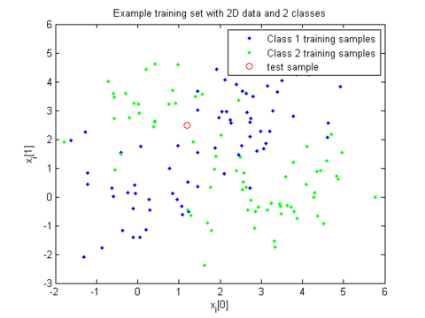
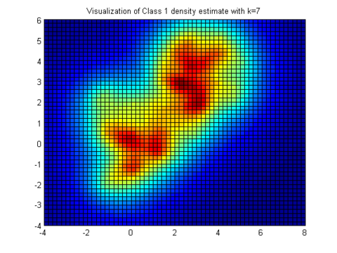
Shown below is a visualization of the density estimate from the above training set with $ \phi(x)=e^{-|x|} $ and k=7.

As a classifier

There are two general methods to use K Nearest neighbors as a classifier.

Method 1: Separately estimate the density and priors for each class

For each class $ c $, you are given a set of $ N_c $ training points $ x_{c1} x_{c2} ... x_{cNc} $ belonging to class c.

You choose a value for K, and a window function separately for each class.

Either estimate the priors as

$  \hat{P}(w_c)=\frac{N_c}{\sum_{i=1}^CN_i}  $

or use some other prior knowledge about the classes.

For each test point $ x_0 $ estimate $ \hat{P}(x_0|w_c) $ as above, and choose the class according to Bayes Rule: the class $ c $ such that $ \hat{P}(x_0|w_c)\hat{P}(w_c) $ is maximized.

Method 2: estimate everything together

Given a training set which is a mixture of the class densities, choose a single K and window function.

For each test point, find a single $ V_k(x_0) $, which is the smallest volume that contains a total of k points from the mixture of classes. (Or a total weight of K, in the case of a window function)

Classify $ x_0 $ as the class with the largest number of points (or largest weight) in the region.

This simplified rule is equivalent to estimating the densities under the assumption that the proportion of samples in the training set of each class is according to the class priors. Because all the class density estimates are using the same window, the volume cancels out. Because the fraction of points in the region is effected by the priors, the number of points of each class in the region takes the priors into account. These together result in the choice of the class with the highest number of points in the region corresponding exactly to the choice of the class with the highest estimated probability $ P(w_c|x_0) $

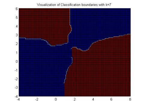
A visualization of the decision boundaries from the above example with k=2 and k=7 shows that larger k results in a smoother boundary.

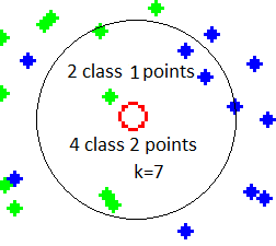
Zooming in on an example of a test point and training set, we can see that the point would be classified as class 2 when k=7

Questions and comments

If you have any questions, comments, etc. please post them on this page.

Back to ECE662, Spring 2014