| Line 92: | Line 92: | ||
A decision making using a classifier based on Parzen window estimation is performed by simple majority voting method. Here, we check how it works. According to Professor Mireille Boutin [2], we pick the class such that <math>Prob(w_{i0}|x_0) \geq Prob(w_i|x_0) \forall i=1,...,c</math> from Bayes' rule. In other words, | A decision making using a classifier based on Parzen window estimation is performed by simple majority voting method. Here, we check how it works. According to Professor Mireille Boutin [2], we pick the class such that <math>Prob(w_{i0}|x_0) \geq Prob(w_i|x_0) \forall i=1,...,c</math> from Bayes' rule. In other words, | ||
| + | <center><math> \begin{array}{cl} | ||
| + | \Longleftrightarrow & \rho(x_0|w_{i0}) Prob(w_{i0} \geq \rho(x_0|w_{i}) Prob(w_{i})\\ | ||
| + | \Longleftrightarrow & \rho(x_0, w_{i0}) \geq \rho(x_0, w_{i}) \\ | ||
| + | \Longleftrightarrow & \displaystyle\sum_{i=1}^n \varphi\left(\frac{\textbf{x}_l - \textbf{x}_0}{h_n}\right) \geq \displaystyle\sum_{i=1}^n \varphi\left(\frac{\textbf{x}_l - \textbf{x}_0}{h_n}\right).\\ | ||
| + | & (\textbf{x}_l$ in class $w_{i0})~~~~~(\textbf{x}_l$ in class $w_{i}) | ||
| + | \end{array}</math></center> | ||
| + | <center> | ||
| + | [[Image:pw_figure4.png|900px]] | ||
| + | Figure 4. The classification error rates with respect to the number of samples from 10 to 1000. | ||
| + | </center> | ||
Revision as of 07:54, 30 April 2014
Parzen window method and classification
A slecture by ECE student Chiho Choi
Partly based on the ECE662 Spring 2014 lecture material of Prof. Mireille Boutin.
in progress....
Unlike parametric density estimation methods, non-parametric approaches locally estimate density function by a small number of neighboring samples [4] and therefore show less accurate estimation results. In spite of their accuracy, however, the performance of classifiers designed using these estimates is very satisfactory.
The basic idea for estimating unknown density function is based on the fact that the probability $ P $ that a vector x belongs to a region $ R $ [1]:
It can be rewritten as
if we assume a small local region $ R $, a large number of samples $ n $, and $ k $ of $ n $ falling in $ R $.
Suppose that the region $ R $ is a $ d $-dimensional hypercube around $ \textbf{x}_i \in \mathbb{R}^n $ in the rest of this slecture, and let the volume $ V_n $:
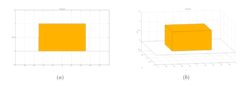
where $ h_n $ is the length of an edge. Then the window function for this hypercube can be defined by
Figure 1. Given window function. (a) where $ d $ = 1, (b) where $ d $ = 2.
We simply shift this window function for $ \textbf{x}_i $ to determine if $ \textbf{x}_i $ belongs to the volume $ V_n $, $ \varphi(\frac{\textbf{x} - \textbf{x}_i}{h_n}) $, and can compute the number of samples $ k_n $ falling in this volume using it:
In Parzen window method, therefore, the estimate for density $ p_n(\textbf{x}) $ is
In order to check how window length effects on $ p_n(\textbf{x}) $, we define $ \delta_n(\textbf{x} - \textbf{x}_i) $ by $ \frac{1}{V_n} \varphi(\frac{\textbf{x} - \textbf{x}_i}{h_n}) $ as an approximation of a unit impulse centered at $ \textbf{x}_i $ [2] and write $ p_n(\textbf{x}) $ [1] by:
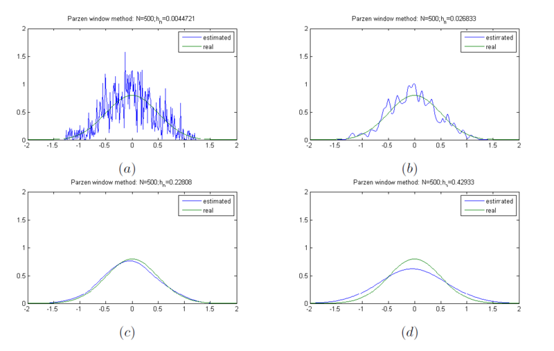
From this observation, we can infer the relationship between $ h_n $ and $ p_n(\textbf{x}) $. If $ h_n $ is very large, the amplitude of $ \delta_n $ is small because $ V_n = h_n^d $. Thus, $ p_n(\textbf{x}) $ becomes a very smooth estimate for $ p(\textbf{x}) $. In contrast, if $ h_n $ is very small, the amplitude of $ \delta_n $ is large. As a result, $ p_n(\textbf{x}) $ is a noisy estimate for $ p(\textbf{x}) $. Therefore, when we have a limited number of samples, to find out an optimal value of $ h_n $ is very important to estimate $ p(\textbf{x}) $. Let us assume that we have an unlimited number of samples. Then, $ V_n $ goes to zero as $n$ increases, and hence $ p_n(\textbf{x}) $ converges to $ p(\textbf{x}) $ [1] no matter what $ h_n $ is.
Figure 2. Density estimate using Parzen window where N = 500. (a) $ h_n $ = 0.0044, (b) $ h_n $ = 0.0268, (c) $ h_n $ = 0.2280, and (d) $ h_n $ = 0.4293.
Figure 3. L2 norm distance between ground truth $ p $ and estimated $ p_n $.
In Figure 2, we can see the effect of the window length on the density estimate results. It demonstrates that a large or small $ h_n $ value causes inaccurate estimation for $ p(\textbf{x}) $. Also, as can be seen in Figure 3, the optimal window length in this experiment can be obtained around 3rd element ($ \textit{i.e.} $, $ h_n $ = 0.23) which shows minimum distance between ground truth $ p $ and estimated $ p_n $. As stated earlier, the choice of $ h_n $ is very important, especially when the number of samples is small.
Since x is a vector of random samples $ \textbf{x}_1, ..., \textbf{x}_n $, $ p_n $ has mean $ E(p_n(\textbf{x})) $ and variance $ Var(p_n(\textbf{x})) $. Thus, $ p_n(\textbf{x}) $ converges to $ p(\textbf{x}) $ [1], if
Let us prove the convergence of the mean and variance [2], respectively.
In order to make this formula converges to zero as n goes to infinity, according to the lecture note [2], we can make $ nV_n \rightarrow \infty $ and $ V_n\rightarrow 0 $ $ (\textit{e.g.}, V_n = \frac{1}{\sqrt{n}} $).
A decision making using a classifier based on Parzen window estimation is performed by simple majority voting method. Here, we check how it works. According to Professor Mireille Boutin [2], we pick the class such that $ Prob(w_{i0}|x_0) \geq Prob(w_i|x_0) \forall i=1,...,c $ from Bayes' rule. In other words,
Figure 4. The classification error rates with respect to the number of samples from 10 to 1000.
Post your slecture material here. Guidelines:
- If you are making a text slecture
- Type text using wikitext markup languages
- Type all equations using latex code between <math> </math> tags.
- You may include links to other Project Rhea pages.
$ \rightarrow $
Questions and comments
If you have any questions, comments, etc. please post them on this page.


