Difference between revisions of "Test" - Rhea

Revision as of 21:05, 14 April 2014

Upper Bounds for Bayes Error
A slecture by Jeehyun Choe

(partially based on Prof. Mireille Boutin's ECE 662 lecture)

1. Introduction

This slecture describes the theoretical upper bounds for Bayes Error. First, in chapter 2, the error bound is expressed in terms of the Bayes classifiers. This error bound expression includes a min function that by using a lemma, the min function can be replaced with the expression of a theoretical error bound. In chapter 3, we specifically derive the Chernoff bound for the Normally distributed data. We also derive the Chernoff distance in the case of Normally distributed data. In section 3.2, some examples for the Chernoff bound are provided.

The materials given in this lecture are based on the lecture notes and the discussions that were shared in Prof. Boutin's ECE662 Spring 2014 course at Purdue University. Examples were designed to reflect the theories taught in the class.

2. Upper Bounds for Bayes Error

2.1 Classifier using Bayes rule

To classify the dataset of feature vectors with C labels, we choose class $w i$ where

\arg\max_{\omega_{i} \in \big\{\omega_{1}, \cdots ,\omega_{c}\big\} } Prob \big( \omega_{i} \mid x \big). \text{......Eq.(2.1)}

However, it is difficult to directly estimate $Prob \big( \omega_{i} \mid x \big)$ . So instead of solving eq.(2.1), we use the Bayes rule to change the problem to

\arg\max_{\omega_{i} \in \big\{\omega_{1}, \cdots ,\omega_{c}\big\} } \rho \big(x \mid \omega _{i}\big) Prob \big( \omega _{i}\big). \text{......Eq.(2.2)}

As can be seen from eq.(2.2), we need to know all the distributions and priors of the classes in the dataset to apply the Bayesian classifier. If the distributions and priors in the dataset is all known, the Bayesian classifier is an optimal classifier since the decision taken following Bayes rule minimizes the probability of error.

2.2 Upper Bounds for Bayes Error

The expected value of the error when deciding following the Bayes rule can be computed as below.

$E \big(error\big) = \int_\Re Prob \big(error \mid x\big) \rho \big(x\big) dx \text{......Eq.(2.3)}$

$= \int_\Re min \big( Prob \big( \omega _{1} \mid x\big), Prob \big( \omega _{2} \mid x\big) \big) \rho \big(x\big) dx \text{......Eq.(2.4)}$

$= \int_\Re min \big( \rho \big( x \mid \omega _{1}\big) Prob \big(\omega _{1}\big) , \rho \big( x \mid \omega _{2}\big) Prob \big(\omega _{2}\big) \big) dx \text{......Eq.(2.5)}$

And we can obtain the upper bound for eq.(2.5) using the following lemma.

min \big\{a, b\big\} \leq a^ \beta b^{1-\beta} \text{......Eq.(2.6)}

where $\forall a,b \geq 0$ and $0 \leq \beta \leq 1$ . Therefore, from eq.(2.5) and (2.6), we can derive the following error bound.

$E \big(error\big) \leq \int_\Re \big( \rho \big(x \mid \omega _{1}\big) Prob \big(\omega_{1}\big) \big) ^ \beta \big( \rho \big(x \mid \omega _{2}\big) Prob \big(\omega_{2}\big) \big) ^{1- \beta } dx = \varepsilon _ \beta \text{......Eq.(2.7)}$

Eq.(2.7) is called Chernoff Bound. This is the error bound that can be computed given the full knowledge of probability of each class.

Since priors are independent of x, we can take priors out of the integral.

$\varepsilon _ \beta = Prob \big(\omega_{1}\big) ^\beta Prob \big(\omega_{2}\big) ^{1-\beta} \int_\Re \rho \big(x \mid \omega _{1}\big) ^ \beta \big( \rho \big(x \mid \omega _{2}\big) \big) ^{1- \beta } dx \text{......Eq.(2.8)}$

For the specific case where $\beta=\frac{1}{2}$ , we call $\varepsilon_{\frac{1}{2}}$ as Bhattacharyya bound.

The smallest of such bound in eq. ...

$S := \min_{\beta \in [ 0,1 ] } \big( \varepsilon _{\beta}\big) \text{......Eq.(2.9)}$

is also sometimes called the Chernoff Bound. This can be used as a error bound since the Bayes error lies somewhere in between 0 and $\min\big( \varepsilon _{\beta}\big)$ .

The Chernoff bound $\varepsilon _{\beta}$ is the probability of error as a function of $β$ . It is usually used for two-category cases and if to be used for multi-category cases, the error bound can be split into several two-category cases and add up all to form the final error bound.

3. Chernoff Bound for Normally Distributed Data

In this section, we will look at the upper bounds for Bayes error in 1-dimensional Normally distributed data.

Assume $\rho \big(x \mid \omega _{1}\big)$ and $\rho \big(x \mid \omega _{2}\big)$ are Gaussians with the distribution

\rho \big(x \mid \omega _{i}\big) = \frac{1}{ \sqrt{2 \pi } \sigma _{i}} \exp \begin{bmatrix} - \frac{1}{2} \big( \frac{x-\mu_{i}}{\sigma_{i}} \big) ^{2} \end{bmatrix}. \text{......Eq.(3.1)}

Since Gaussian distribution is one of the exponential families, eq.(3.1) can be expressed as a following form [1] [3].

\rho \left(x\mid {\omega}_{i} \right) = \exp\left(<t\left(x \right), \theta > -F\left(\theta \right)+k\left(x \right)\right) \text{......Eq.(3.2)}

where $t\left(x \right)$ is sufficient statistic and $θ$ is parameters.

It is easier to derive the Chernoff Bound for Normally distributed data if we use the form in eq.(3.2). Therefore, we will first find the exponential form of the Gaussian distribution in eq.(3.1).

\rho \left(x\mid {\omega}_{i} \right) = \exp \begin{bmatrix} \ln \big( \frac{1}{ \sqrt{2 \pi } \sigma _{i}} \big) \end{bmatrix} \exp \begin{bmatrix} - \frac{1}{2} \big( \frac{x-\mu_{i}}{\sigma_{i}} \big) ^{2} \end{bmatrix} \text{......Eq.(3.3)}

= \exp \begin{bmatrix} \frac{1}{2} \ln \big( \frac{1}{ 2{\sigma}^{2}_{i}\pi } \big) - \frac{1}{2} \big( \frac{x^{2} -2\mu_{i}x + \mu_{i}^{2}}{\sigma_{i}^{2}} \big) \end{bmatrix}

= \exp \begin{bmatrix} \frac{1}{2} \ln \left(\frac{1}{2\sigma _{i}^{2}} \right) - \frac{1}{2} \ln \pi - \frac{x^{2}}{2\sigma _{i}^{2}} + \frac{x \mu_{i}}{\sigma _{i}^{2}} - \frac{\mu_{i}^{2}}{2\sigma _{i}^{2}} \end{bmatrix}

\rho \left(x\mid {\omega}_{i} \right) = \exp \begin{bmatrix} \underbrace{ - \frac{x^{2}}{2\sigma _{i}^{2}} + \frac{x \mu_{i}}{\sigma _{i}^{2}} }_{< t\left(x \right), \theta_{i} >} + \underbrace{ \frac{1}{2} \ln \left(\frac{1}{2\sigma _{i}^{2}} \right) - \frac{1}{2} \ln \pi - \frac{\mu_{i}^{2}}{2\sigma _{i}^{2}} }_{-F\left(\theta_{i} \right)} \end{bmatrix} \text{......Eq.(3.4)}

From eq.(3.4), we can set the sufficient statistic $t\left(x \right)$ and parameters $θ i$ as

t\left(x \right) = \left(x, -x^{2} \right) \text{......Eq.(3.5)}

\theta_{i} = \left(\frac{\mu_{i}}{\sigma_{i}^{2}} , \frac{1}{2\sigma_{i}^{2}}\right). \text{......Eq.(3.6)}

We can also express $F\left(\theta_{i} \right)$ and $k\left(x \right)$ as

F\left(\theta _{i} \right) = \frac{\theta _{i,1} ^{2}}{4\theta_{i,2}} -\frac{1}{2}\ln\theta _{i,2}+\frac{1}{2}\ln\pi \text{......Eq.(3.7)}

k\left(x \right) = 0 \text{......Eq.(3.8)}

where $θ i,1$ and $θ i,2$ refer to the first and second components in eq.(3.6).

Now by substituting this exponential form of Gaussian densities into eq.(2.8), we can derive the simpler formula of Chernoff bound.

3.1 Derivation of Chernoff Distance

Let the integral part in eq.(2.8) be the Chernoff $β$ -coefficient [3].

$\int_\Re \rho \big(x \mid \omega _{p}\big) ^ \beta \big( \rho \big(x \mid \omega _{q}\big) \big) ^{1- \beta } dx = \int_\Re [ \exp \left( < t\left(x \right), \theta_{p} > -F\left(\theta_{p} \right) \right) ]^{\beta} [ \exp \left( < t\left(x \right), \theta_{q} > - F\left(\theta_{q} \right) \right) ]^{1-\beta} dx \text{......Eq.(3.9)}$

= \int_\Re \exp \left( < t\left(x \right), \beta\theta_{p} > -\beta F\left(\theta_{p} \right) \right) \exp \left( < t\left(x \right), \left(1-\beta \right)\theta_{q} > -\left(1-\beta \right) F\left(\theta_{q} \right) \right) dx

= \int_\Re \exp \left( < t\left(x \right), \beta\theta_{p} > + \left( < t\left(x \right), \left(1-\beta \right)\theta_{q} > -\beta F\left(\theta_{p} \right) \right) -\left(1-\beta \right) F\left(\theta_{q} \right) \right) dx

= \int_\Re \exp \left( < t\left(x \right), \beta\theta_{p} + \left(1-\beta \right)\theta_{q} > \underbrace{ -\beta F\left(\theta_{p} \right) -\left(1-\beta \right) F\left(\theta_{q} \right) }_{ \text{independent of x} } \right) dx

= \exp \left( -\beta F\left(\theta_{p} \right) -\left(1-\beta \right) F\left(\theta_{q} \right) \right) \int_\Re \exp \left( < t\left(x \right), \beta\theta_{p} + \left(1-\beta \right)\theta_{q} > \right) dx

\begin{array}{l} = \exp \left( -\beta F\left(\theta_{p} \right) -\left(1-\beta \right) F\left(\theta_{q} \right) \right) \exp \left( F \left( \beta \theta_{p} + \left( 1-\beta \right) \theta_{q} \right) \right) \\ \times \underbrace{ \int_\Re \exp \left( < t\left(x \right), \beta\theta_{p} + \left(1-\beta \right)\theta_{q} > \right) \exp \left( - F \left( \beta \theta_{p} + \left( 1-\beta \right) \theta_{q} \right) \right) dx }_{=1} \end{array} \text{......Eq.(3.10)}

= \exp \left( -\beta F\left(\theta_{p} \right) -\left(1-\beta \right) F\left(\theta_{q} \right) + F \left( \beta \theta_{p} + \left( 1-\beta \right) \theta_{q} \right) \right) \text{......Eq.(3.11)}

We can see that eq.(3.11) is in the form $e^{ -k \left( \beta \right) }$ . $k \left( \beta \right)$ is sometimes called Chernoff distance. To obtain the formula for $-k \left( \beta \right)$ , we can substitute $F\left( \right)$ terms in eq.(3.11) with the expression in terms of $\mu_{i}$ or $\sigma_{i}$ using eq.(3.6) and eq.(3.7).

\begin{cases} \beta F\left(\theta_{p} \right) = \beta\frac{\mu_{p}^{2}}{2\sigma_{p}^{2}}-\beta\frac{1}{2}\ln\left(\frac{1}{2\sigma_{p}^{2}} \right)+\beta\frac{1}{2}\ln\pi \\ \left(1-\beta \right) F\left(\theta_{q} \right) = \left(1-\beta \right) \frac{\mu_{q}^{2}}{2\sigma_{q}^{2}}-\left(1-\beta \right)\frac{1}{2}\ln\left(\frac{1}{2\sigma_{q}^{2}} \right)+\left(1-\beta \right)\frac{1}{2}\ln\pi \\ - F \left( \beta \theta_{p} + \left( 1-\beta \right) \theta_{q} \right) = - F \left( \theta_{tot} \right) \end{cases} \text{......Eq.(3.12)}

The last line in eq.(3.12) can be computed by first finding the $θ t' o' t$ as

\theta_{tot} = \beta\left(\frac{\mu_{p}}{\sigma_{p}^{2}}, \frac{1}{2\sigma_{p}^{2}} \right) + \left(1-\beta \right)\left(\frac{\mu_{q}}{\sigma_{q}^{2}}, \frac{1}{2\sigma_{q}^{2}} \right) = \left( \frac{ \beta \mu_{p}\sigma_{q}^{2}+\left(1-\beta \right)\mu_{q}\sigma_{p}^{2} }{\sigma_{p}^{2}\sigma_{q}^{2}} , \frac{ \beta\sigma_{q}^{2}+\left(1-\beta \right)\sigma_{p}^{2} }{2\sigma_{p}^{2}\sigma_{q}^{2}} \right)

and subtituting this result into the eq.(3.7) as follows:

- F \left( \theta_{tot} \right) = -\frac{[\beta \mu_{p}\sigma_{q}^{2}+\left(1-\beta \right)\mu_{q}\sigma_{p}^{2} ]^{2}}{ 2\sigma_{p}^{2}\sigma_{q}^{2} \left(\beta\sigma_{q}^{2}+\left(1-\beta \right)\sigma_{p}^{2} \right)} + \frac{1}{2}\ln\frac{\beta\sigma_{q}^{2}+\left(1-\beta \right)\sigma_{p}^{2} }{2\sigma_{p}^{2}\sigma_{q}^{2}} - \frac{1}{2}\ln\pi.

Therefore, $k \left( \beta \right)$ can be derived as follows:

\begin{array}{c} k \left( \beta \right) = \beta F\left(\theta_{p} \right) + \left(1-\beta \right) F\left(\theta_{q} \right) - F \left( \theta_{tot} \right) \end{array} \text{......Eq.(3.13)}

= \beta\frac{\mu_{p}^{2}}{2\sigma_{p}^{2}}+\left(1-\beta \right) \frac{\mu_{q}^{2}}{2\sigma_{q}^{2}} -\frac{\left[\beta \mu_{p}\sigma_{q}^{2}+\left(1-\beta \right)\mu_{q}\sigma_{p}^{2} \right]^{2}}{ 2\sigma_{p}^{2}\sigma_{q}^{2} \left(\beta\sigma_{q}^{2}+\left(1-\beta \right)\sigma_{p}^{2} \right)} + \frac{1}{2}\ln\left[\frac{\beta\sigma_{q}^{2} + \left(1-\beta \right)\sigma_{p}^{2} }{\left( \sigma_{p}^{1-\beta}\sigma_{q}^{\beta}\right)^{2}} \right]

k \left( \beta \right) = \frac{\beta\left(1-\beta \right)\left(\mu_{p}-\mu_{q} \right)^{2} }{2 \left(\beta\sigma_{q}^{2}+\left(1-\beta \right)\sigma_{p}^{2} \right)} + \frac{1}{2}\ln\left[ \frac{\beta\sigma_{q}^{2} + \left(1-\beta \right)\sigma_{p}^{2} } {\sigma_{p}^{2 \left(1-\beta \right) }\sigma_{q}^{2\beta}} \right]. \text{......Eq.(3.14)}

Therefore, the error bound would be

\varepsilon _ \beta = Prob \big(\omega_{1}\big) ^\beta Prob \big(\omega_{2}\big) ^{1-\beta} \exp \left[ -k \left( \beta \right) \right]. \text{......Eq.(3.15)}

3.2 Example

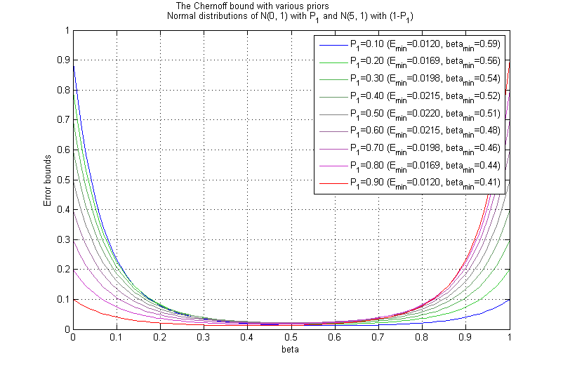
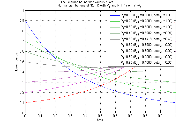
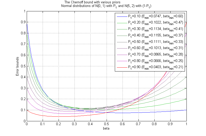
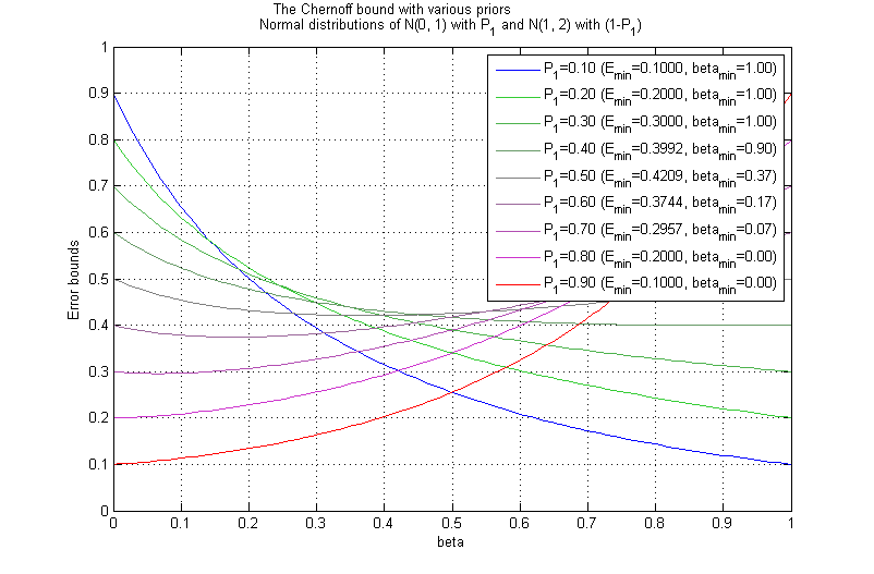
By using the closed form equation of the Chernoff bound shown in eq.(3.14) and eq.(3.15), we can visualize several examples of Chernoff bounds for Normally distributed data.

Figure 3.1: Chernoff bound for N(0,1) and N(5,1)

In figure 3.1, we can see that the Chernoff bound is generally low, since the gap between the two means is high compared to the variances. The Chernoff bound doesn't change much as the prior changes from 0.1 to 0.9 in this case.

Figure 3.2: Chernoff bound for N(0,1) and N(1,1)

Figure 3.2 shows the case where the gap between two means is low compared to the variances. In this case, as the prior for one category gets larger than the other prior, the Chernoff bound goes down. However, when both priors have similar values, the Chernoff bound gets higher.

We can observe that both in figure 3.1 and figure 3.2, the Chernoff bound is close to the Bhattacharyya bound when the Priors have the equal values.

Figure 3.3: Chernoff bound for N(0,1) and N(5,2)

Figure 3.4: Chernoff bound for N(0,1) and N(1,2)

Figure 3.3 and figure 3.4 show the cases when the variances of two categories differ. In previous examples where the variance for both categories are the same, the Chernoff bound was close to the Bhattacharyya bound when the Priors have the equal values. However, figure 3.3 and figure 3.4 don't show such patterns.

Summary

In this lecture, we have shown how the Chernoff bound can be derived. We have derived the Chernoff bound in a closed form for the 1D Gaussian distributions. We also saw some examples of the Chernoff bounds on different sets of Normally distributed 1-dimensional data.

Reference

[1] C. A. Bouman. A Guide to the Tools of Model Based Image Processing. Purdue University, 2013.

[2] R. O. Duda, P. E. Hart, and D. G. Stork. Pattern Classification (2nd Edition). Wiley-Interscience, 2000.

[3] F. Nielsen. Chernoff information of exponential families. ArXiv e-prints, 2011.

Questions and comments

If you have any questions, comments, etc. please post them On this page.

Back to Spring 2014 ECE662 page

@@ Line 1: / Line 1: @@
 <center><font size="4"></font>
 <font size="4">'''Upper Bounds for Bayes Error''' <br> </font> <font size="2">A slecture by Jeehyun Choe</font>
@@ Line 4: / Line 6: @@
 <font size="2">(partially based on Prof. [https://engineering.purdue.edu/~mboutin/ Mireille Boutin's] ECE [[ECE662|662]] lecture) </font>
 </center>