Contents
[hide]Filtering
By Dhruv Lamba.
Introduction
Filtering in a broad sense, is a method of removing any unwanted quantity from a mixture of the desired quantity and the undesired quantity. In the world of signals, this generally applies to the process of either separating different channels of a signal, or removing a noise signal to get the original signal.
This usually makes more sense when we talk about something real. Say, music, or images, or surprisingly, even the stock market! That's right. It is possible, from simple spectral analysis to "filter" out long-term and short term trends from any time varying data. This includes weather, astronomical events, and pretty much any time-varying signal you can think of.
Simple Example
- I always like to start out with our friendly sine wave. After all, that is what Fourier started with too.
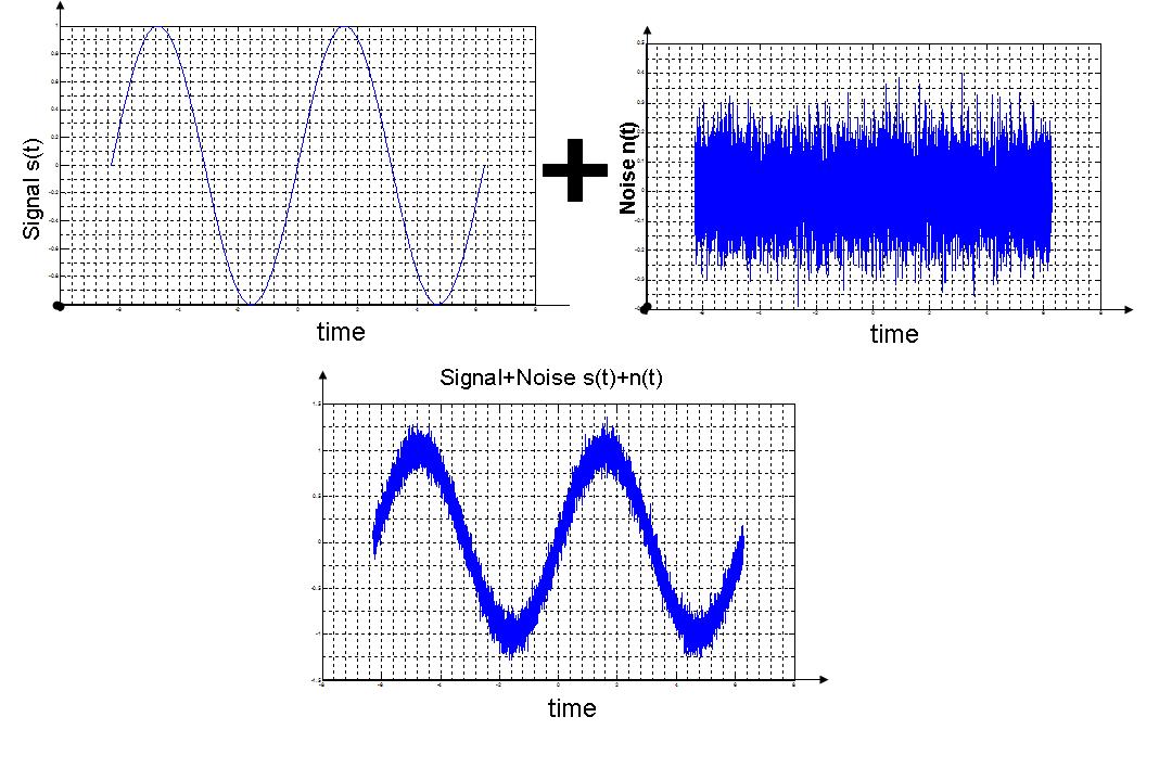
- So, what we do is start by taking a clean sine wave from -2pi to 2pi
- To the sine wave, we add some pretty ugly Gaussian noise, shown above.
- What results is a much noisier signal, as can be clearly seen.
To try this yourself, you can plop the following in an m-file
clear all;
close all;

clc;

t = [-2*pi:.1:2*pi];
signal = sin(t);
plot(t,sin(t));
grid minor;

noise = randn(1,length(t));
noise = noise/10;
figure;
plot(t,noise);
grid minor;

mixed = noise + signal;
figure;
plot(t,mixed)
grid minor;
- Now if someone presented us an ugly signal like that, we can without panicking, get the original signal back
- How? LOW PASS FILTER
- However, a Low Pass Filter isn't a magic device that removes noise
- It needs to have well defined cut off frequencies and pass-band gains.
- To understand this better, let us see how our signals look in the frequency domain
- To do this, we take the original signal's FFT (this will be an N point FFT where N = 126 because we have an interval of -2pi or -6.283 to 2 pi or 6.283 at intervals of .1, Hence 126 samples and we know that N samples will yield N points in the FFT)
- An important thing to remember is that the frequency corresponding to the kth sample is actually $ 2pik/N $
To try these figures, you may use the following code in continuation with the previous code above:
k = -63:62;

figure;
plot(k,fftshift(abs(fft(signal))));
grid;
axis([min(k),max(k),0,63]);

figure;
plot(k,fftshift(abs(fft(mixed))));
grid;
axis([min(k),max(k),0,63]);
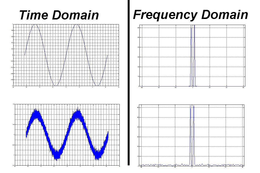
- The first thing to note from the figure is that the signal with no noise has a frequency spectrum like we expected, two nice clean impulses corresponding to it's natural frequency.
- On the other hand, the spectrum of the sin wave with added noise, has a good deal of frequency components outside the natural frequency, and since the noise we added was Gaussian instead of a single frequency, it's all over the spectrum.
- To remove the noise, we need to remove the frequency components that correspond to it in the Fourier Domain
- The problem however is, that since the noise affects all regions of the spectrum, removing it's frequency components, or conversely preserving the original signal's components, will not remove the noise completely.
- Still, let's see the best that can be done.
Low Pass Filter
- Again, the objective is to design a low pass filter that keeps the frequency components of the original signal and kills everything else.
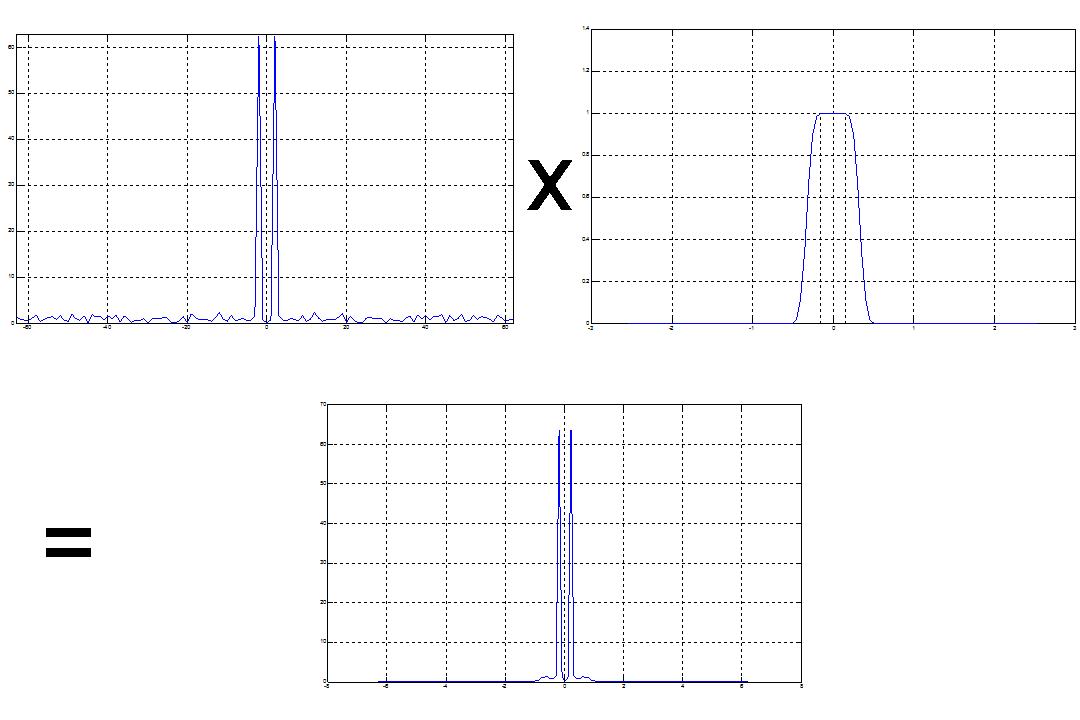
- To visualize this, think of multiplying a box
$ H(\omega) = \left\{ \begin{array}{c l} A &\omega \in [-w_0,w_0]\\ 0 & \omega\not\in [-w_0,w_0] \end{array} \right. $
with the frequency domain of the signal to be filtered, so that what results (ideally) is
$ X(\omega) = \left\{ \begin{array}{c l} AX(\omega) &\omega \in [-w_0,w_0]\\ 0 & \omega\not\in [-w_0,w_0] \end{array} \right. $
- Of course, filters are not ideal in the real world, and instead of a constant A in the pass-band, we get a reasonably constant function of w in the pass band and a severely attenuated $ \epsilon $ as the gain for the stop band, where $ \epsilon ->0 $
Filters in MATLAB
- So, let's see how good we can make our filters, so that they meet the specifications above.
- Now even though MATLAB lets us make hundreds of types of filters, I like using the Parks Mc Clellen FIR filter.
- There are two reasons for this, (1) I used this filter extensively in a summer research project and grew to know and love it well, and 2) the Parks Mc Clellen filter is an equiripple filter which means that the ripples in the pass band and stop band are equal. Why this is good is beyond the scope of this page. But it is good, trust me, and they are hence called optimal filters.
- Coming back to our example, the following code may be used to generate a 100 point Equiripple FIR filter
freq = 1/(2*pi);
sample_rate = 1/.1;
steep = 1;

h = firpm(100,[0 freq/(.5*sample_rate) (freq+steep)/(.5*sample_rate) 1],[1 1 0 0]);
- Here, freq is the cut-off frequency, which in our case is $ \pm 1/2 \pi $. To understand why this is true, consider the fact that sin(t) will have a natural frequency of $ 1/2 \pi $ and hence the two impulses in the frequency domain will be at $ \pm 1/2 \pi $
- However, a disclaimer here; we do not want our filter to be aggressive. That is, we don't want it to obliterate everything outside$ \pm 1/2 \pi $. What we want instead is a nice roll-off, which makes sure that frequencies close to the cut-off are cut-off evenly and not drastically.
- So, we introduce a steepness variable, that controls the roll-off called steep.
- The sampling rate is simply 10 because we know that the original sine wave is constructed using points every 0.1 units.
- This FIR is really easy to build because it basically scales the DTFT $ \omega $ axis of [0 , $ \pi $ to [0 to 1] and hence we can get a pretty good low pass by simply scaling the w axis of our desired filter to [0, 1]
- The results of the frequency domain multiplication with the filter (CONVOLUTION IN THE TIME DOMAIN) gives us the desired signal without noise.
- It is worth noting that there are some extra frequency contents in the 0 to $ \pm 1/2 \pi $ range, but these were expected, because the filter removed everything except that range.
- This is a necessary evil, but the good news is that most of the noise in the spectrum is gone! :)
- So everything looks good in the frequency domain and the world is a happy place again
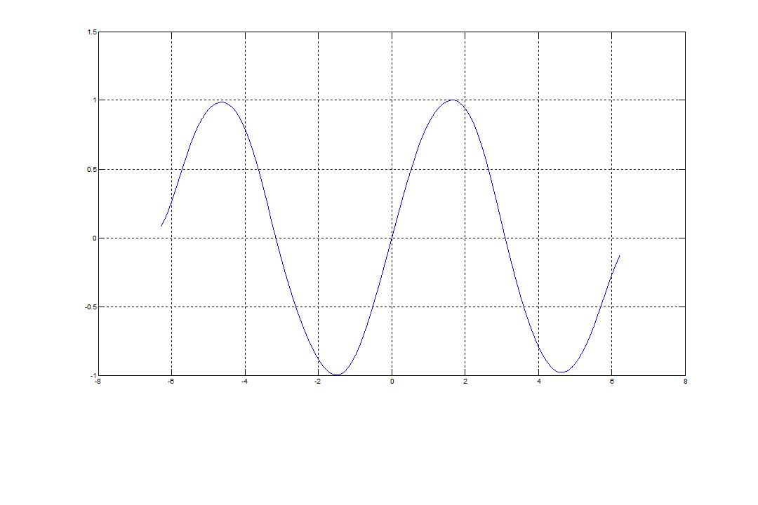
- As a final check let's see how close to the original the time domain signature looks
- Not too bad, I would say. The curve is a little squiggly and the amplitude messed up a bit, but compared to the noisy blob of sine we saw above, it's an award-winner.
- Here's some try it yourself:
copyright Dhruv Lamba

figure;

f=[-50:50]*1/(pi*2*pi);

plot(f,fftshift(abs(fft(h))));

line([1/(2*pi) 1/(2*pi)],[0 1],'Linestyle',':','Color',[0 0 0 ]);
line([-1/(2*pi) -1/(2*pi)],[0 1],'Linestyle',':','Color',[0 0 0]);

grid on;


filtered = conv(h,mixed);
filtered = filtered(51:176);

figure;
plot(t,filtered);
grid

figure;
plot(t,fftshift(abs(fft(filtered))));
grid;


