Classification using Bayes Rule in 1-dimensional and N-dimensional feature spaces
A slecture by Jihwan Lee
Partly based on the ECE662 Spring 2014 lecture material of Prof. Mireille Boutin.
Contents
Introduction
In this slecture, we discuss Bayes rule that is widely used for many different kinds of applications, especially, pattern recognition. Due to its simplicity and effectiveness, we can use the method in both discrete values case and continuous values case, and it also usually works well in multi-dimensional feature space. So, we will take a look at what the definition of Bayes rule is, how it can be used for the classification task with examples, and how we can derive it in different cases.
Bayes' Theorem
Bayes theorem is a probabilistic theory that can explain a relationship between the prior probability and the posterior probability of two random variables or events. Give two events $ A $ and $ B $, we may want to know $ P(A|B) $ and it can be obtained if we know knowledge for other probabilities, $ P(B|A) $, $ P(A) $, and $ P(B) $. By the definition of the conditional probability, a joint probability of $ A $ and $ B $, $ P(A, B) $, is the product of $ P(A|B) $$ P(B) $. We can also write $ P(A, B) = P(B|A)P(A) $. From those two equations, $ P(A|B)P(B) = P(B|A)P(A) $ and we can conclude
The formula above is called Bayes Theorem. Let's see an example. Suppose that a man told you that he had a nice conversation with a person. Assuming the populations of male and female are the same, the probability that his conversational partner was a woman is 0.5. However, if he gives you additional information that the conversational partner had long hair, then the probability of the partner being a woman will be higher than 0.5 because women are more likely to have long hair. So, let $ W $ be an event that the conversational partner was a women and $ L $ be an event that a person has a long haired person. Suppose that 75% of all women have long hair, 15% of men have long hair, and both genders are equally likely. That is, $ P(L|W)=0.75, P(W)=P(M)=0.5 $, and these are what we already know. With these information, we can say that the probability that the person who he had a conversation with was a woman is
$ \begin{align} P(W|L) & = \frac{P(L|W)P(W)}{P(L|W)P(W) + P(L|M)P(M)} \\ & = \frac{0.75 * 0.5}{0.75*0.5 + 0.15*0.5} \\ & = \frac{5}{6} \simeq 0.83 \end{align} $
The probability that the conversational partner was a woman has changed from 0.5 to 0.83 after we get additional information that the partner was a long-haired person. By introducing the new information, we can narrow down the sample place, that is, from whole population to only a group of people who have long hair. Thus, since women are more likely to have long hair, the probability could be increased.
Here is another example. In a public university, 51% of the students are males. One adult is randomly selected for a survey. It turned out later that the selected survey subject was studying sciences. Also, 10% of students study sciences while 5% of females study sciences. What is the probability that the selected subject is a male? Let's use the following notations:
- $ M $ = male
- $ \overline{M} $ = female
- $ S $ = study sciences
- $ \overline{S} $ = study other fields
- $ M $ = male
Before having the information about the subject's major, the probability that the subject is a male is 51%, that is, $ P(M) = 0.51 $. However, based on the additional information, we now have the following:
- $ P(M) = 0.51 $ because 51% of students are males
- $ P(\overline{M}) = 0.49 $ because 49% of students are females
- $ P(S|M) = 0.1 $ because 10% of the male students study sciences
- $ P(S|\overline{M}) = 0.05 $ because 5% of the female students study sciences
- $ P(M) = 0.51 $ because 51% of students are males
Now, in order to figure out the probability that the survey subject is a male given the subject studies sciences, $ P(M|S) $, we can apply Bayes theorem as following
In this example, the sample space we have to consider could be reduced from whole population to people who study sciences by obtaining additional information. This change could affect the probability of the survey subject being a male. And the conditional probability $ P(M|S) $ can be obtained easily by using Bayes rule once we have known other probabilities, $ P(M) $, $ P(S) $, and $ P(S|M) $.
Classification by Bayes Rule
In this section, we investigate how Bayes rule can be used for the task of classification. Suppose that there are many classes $ \omega_1, \omega_2, \dots, \omega_c $ and data that should belong to one of those classes. So, what we want to do is to classify new data that do not have any class information into one of the classes, based on training data whose class membership information is already known. Using Bayes rule, the probability that a new data $ x $ belongs to class $ \omega_i $ is given by
$ \begin{align} P(\omega_i | x) & = \frac{\rho(x|\omega_i)P(\omega_i)}{\rho(x)} \\ & = \frac{\rho(x|\omega_i)P(\omega_i)}{\sum_{l=1}^{c}\rho(x|\omega_l)P(\omega_l)} \end{align} $
where $ \rho $ is a density function for continuous values. That is, $ \rho(x|\omega_i) $ is a class-conditional density, $ P(\omega_i) $ is a prior probability, $ \rho(x) $ is an evidence which can be usually ignored, and $ P(\omega_i|x) $ is a posterior probability. Now we can compare probability values of $ P(\omega_i|x) $ for each class and make a decision by taking one with higher probability as following
From now on, we consider only two class classification problem for simplicity. Let $ g_1(x)=\rho(x|\omega_1)P(\omega_1) $ and $ g_2(x)=\rho(x|\omega_2)P(\omega_2) $. Then we can decide class $ \omega_1 $ for $ x $ if $ g_1(x) \geq g_2(x) $, otherwise, decide class $ \omega_2 $. Equivalently, we can define a discriminant function $ g(x) = g_1(x) - g_2(x) $ and decide class $ \omega_1 $ if $ g(x) \geq 0 $, otherwise class $ \omega_2 $. We here need to notice followings
- The discriminant function $ g(x) $ is not unique. As long as the discriminant function is monotonically increasing, it will make the same decision. (e.g., $ g(x) = \ln{g_1(x)} - \ln{g_2(x)} $)
- We do not need to know the actual function $ g(x) $, but need to know just its sign.
Then what is the expected value of the error when we make decision by following Bayes rule?
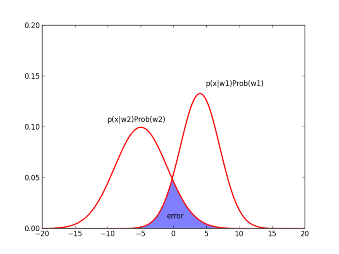
Note that $ g(x) = 0 $ has at most 2 solutions, which means that those two distributions for $ \omega_1 $ and $ \omega_2 $ have one intersection or two intersections. Let's see the case of one intersection at the point $ t $.
Let $ y_2 = \frac{x-\mu_2}{\sigma_2}, y_1 = \frac{x-\mu_1}{\sigma_1} $, and $ \Phi(\alpha) = \int_{-\infty}^{\alpha}{\frac{1}{\sqrt{2 \pi}} e^{- \frac{x^2}{2}} dx} $. Then,
In Figure 1, the shaded region represents the probability that data would be misclassified, that is, error. Let $ t $ be an intersection point. Based on Bayes rule, we should classify all data on the left of $ t $ into $ \omega_2 $, and all other data that are on the right of $ t $ will be classified into $ \omega_1 $. Therefore, as the region is larger, in other words, two distributions share larger overlapped area, the expected error will be increasing.
The following sections describe two cases of classification. One is where data exist in 1-dimensional feature space and the other is where data exist in N-dimensional feature space.
Case 1: 1-dimensional feature space
For simplicity, samples $ x_i $ of class $ \omega_i $ are drawn from Gaussian distribution $ x_i \sim N(\mu_i, \sigma_i^2) $. Then, the class-conditional density is given by
and let's take
where $ C_i $ is a constant value which is independent of $ x $. Finally, we can use the following discriminant function
So, given a value of $ x $, we can assign class to $ x $ based on the sign of the discriminant function above, i.e., if $ g(x) \geq 0 $ then $ x $ should be class $ \omega_1 $.
Case 2: N-dimensional feature space
Let's assume that each data is drawn from Multivariate Gaussian distribution with mean $ \mu_i $ and standard deviation matrix $ \Sigma_i $. Then the class-conditional density is given by
Again we use
Note that the first term is actually $ -\frac{1}{2} $ square of Mahalanobis distance from $ \vec{x} $ to $ \vec{\mu_i} $ and the remaining terms are independent of $ \vec{x} $, which means that the closer $ \vec{x} $ is to $ \vec{\mu_i} $, the larger $ g_i(x) $ is. We can also observe that if the standard deviation matrix $ \Sigma $ is equal to $ I $(identity matrix) the Mahalanobis distance at the first term of the equation above becomes Euclidean distance, that is,
and the second term can be ignored since it is constant and independent of $ \vec{x} $ In two-class classification, we should decide $ \omega_i $ if
otherwise, we should decide $ \omega_2 $. One interesting observation here is that making decisions will be based on a linear separation, which is a hyperplane. The hyperplane can be defined by a set of points which are equidistant to $ \mu_1 $ and $ \mu_2 $ if all priors are equal($ P(\omega_i) = \frac{1}{c} \forall i = 1, \dots, c $). Thus, for a given data $ x $, we can choose a class that has a nearest mean from $ x $. Let's see the following derivation:
The formula for a hyperplane is $ n \cdot x + b = 0 $ where $ n $ is a normal vector. Thus, the equation above can be representing a hyperplane and the normal vector is $ n = \vec{\mu_i} - \vec{\mu_j} $.
We can also consider another case where each class $ \omega_i $ has the same covariance matrix $ \Sigma $, that is, $ \Sigma_i = \Sigma_j $. Then $ g_i(x) $ is given as follows,
For this case, the decision boundaries are still hyperplanes, but they may no longer be normal to the lines between the respective class means $ \vec{\mu_i} $ and $ \vec{\mu_j} $.
The other possible case is where there are different covariance matrices for each class, which is actually the most general case. If each class $ \omega_i $ has its own arbitrary covariance matrix $ \Sigma_i $, then $ g_i(x) $ should be as follows,
So if we let $ g_1(\vec{x}) = g_2(\vec{x}) $, the resulted equation will be a quadratic function of $ \vec{x} $. Therefore, the decision boundaries are quadratic, specifically, hyperellipses.
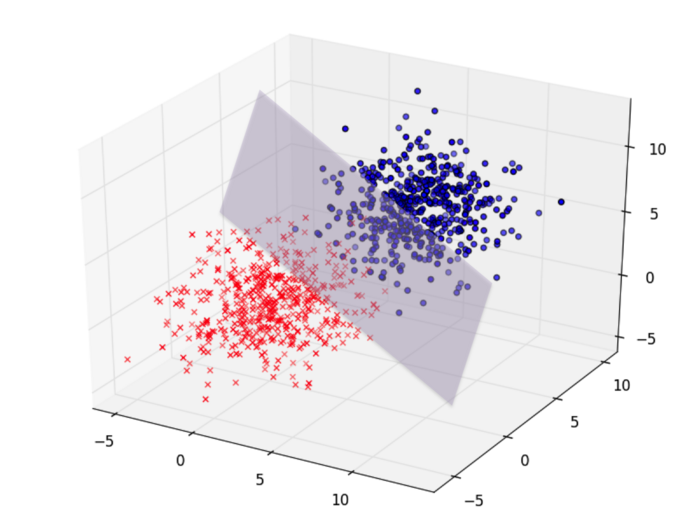
Figure 2 shows classification in three dimensional feature space. If data are drawn from Gaussian distributions with the identity covariance matrices, then the decision boundary between those two classes becomes a hyperplane and its normal vector should be $ \vec{\mu_1} - \vec{\mu_2} $.

Conclusion
In this slecture, we have discussed not only the basic principle of Bayes rule with simple examples but also how it can be used for the task of classification, and we have investigated at how to classify normally distributed data in 1-dimensional and N-dimensional feature spaces. Despite the simplicity of Bayes rule, it is greatly effective and efficient, and it works well for various types of data. Also its optimality has been already proved. As long as we assume that given data to classify follow Gaussian distribution, we can define a simple discriminant function as shown above. In order to make this classification method produce more accurate results, one critical issue is density estimation. In most cases, it may be impossible to know the actual densities over whole data. So we need to estimate class-conditional densities or probabilities and prior probabilities. If data are normally distributed, then we can make the issue easier by estimating sample means and standard deviations. Actually, a lot of density estimation techniques have been proposed but they are beyond the main topic in this slecture. For someone who is interested in it, we can refer to other slectures talking about Maximum Likelihood Estimation, Bayesian Parameter Estimation, Parzen window method, k-nearest neighbor, and so on. One related and interesting problem needed to further investigate is how well Bayes rule classification works for non-normally distributed data. In fact, most data we should classify in real world do not follow Gaussian distribution and sometimes we do not know even their underlying distributions. Thus, it is sometimes infeasible to directly use the discriminant functions we defined above. This problem is remained as follow-up discussion.
References
[1] Mireille Boutin, “ECE662: Statistical Pattern Recognition and Decision Making Processes,” Purdue University, Spring 2014
[2] Mario F. Triola, http://faculty.washington.edu/tamre/BayesTheorem.pdf
[3] Richard O. Duda, Peter E. Hart, David G. Stork, "Pattern Classification", 2nd Edition
Questions and comments
If you have any questions, comments, etc. please post them on this page.


