In class, we covered the simple Bayesian classifier. This form of classification falls under a category known as supervised learning. What this means is that a set of labelled data data is used to to "train" the underlying model. However, it is not always possible to have such a data set, yet we may still wish to discover some form of underlying structure in an unlabelled data set. Such a task falls under the category of unsupervised learning.

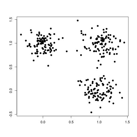
Clustering is a form of unsupervised learning. Clustering is the problem of identifying groups, or clusters of data points in multidimensional space. For example, consider the following data set:

Figure 1

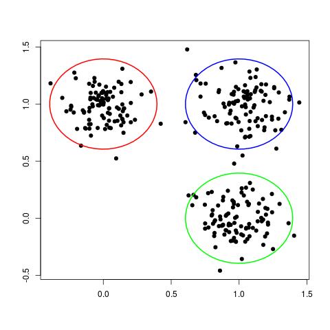
Although this data set is not labelled, we can still clearly see three different groups, or clusters, of data points, as shown here:

Figure 2

In some ways, each cluster can be thought of a different "class" of data points. In this way, clustering can be seen as the unsupervised analog of the classification problem.

There is no "best" clustering algorithm. Any algorithm imposes some sort of structure on the data. If the structure imposed by the clustering algorithm matches the true structure of the data, then the actual clusters may be discovered. As a result, there are many different clustering methods. Here I will describe a popular and intuitive method known as K-means clustering.

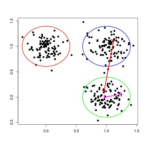
One way of thinking about a cluster is a set of points who's pairwise distances are small compared to the distance to the points of a different cluster. This is illustrated in the following figure:

Figure 3

In the figure above, the magenta line represents a general distance between two points of the same cluster and the red line represents a general distance between points of different clusters. Intuitively, we expect the red line to be significantly longer than the magenta line.

The K-means algorithm formalizes this by first introducing a set of $ D $-dimensional vectors, $ \mu_k $, where $ k = 1,...,K $. These vectors represent the current guess for the center of each cluster. As you will see later, throughout the k-means algorithm, we optimize the locations of these centers and the assignment of data points to specific clusters.

The K-means algorithm also introduces a set of binary variables to represent assignment of data points to specific clusters:
$ r_{nk} \in \{0,1\} $
where $ k = 1,...,K $ and $ n = 1,...,N $ and $ N $ is the total number of data points.
This set of binary variables is interpreted as follows: if data point $ n $ is assigned to cluster $ k $, then $ r_{nk} = 1 $, otherwise $ r_{nk} = 0 $.

Now, given a set of data points $ \{X_1,...,X_N\} $, we can define a cost function:

What this represents is the sum of squares of the distance of each data point to it's assigned vector $ \mu_k $. To see this, notice that since $ r_{nk} = 1 $ only when point $ n $ has been assigned to cluster $ k $, that is the only distance that gets added to our total cost function. All other combinations of $ n $ and $ k $ lead to $ r_{nk} = 0 $, and thus do not affect the total cost function, $ J $.

The K-means algorithm finds a local minimum of this cost function by the following steps:

1. Choose starting locations for $ \mu $.
2. Minimize $ J $ with respect to $ r $, keeping $ \mu $ constant.
3. Minimize $ J $ with respect to $ \mu $, keeping $ r $ constant.
4. Repeat steps 2 and 3 until the value of $ J $ no longer changes

Step 1: Choose starting locations for $ \mu $

This step is perhaps both the easiest to understand and hardest to implement in a "good" way. At it's most basic level, all we need to do is choose starting locations for the cluster centers ($ \mu $). Any random starting locations will work, but some configurations may lead to poor results after the K-means algorithm terminates.

Step 2: Minimize $ J $ with respect to $ r $, keeping $ \mu $ constant

The terms in $ J $ for each $ n $ are independent of each other, so the optimization is rather simple. Assign each data point to the center that gives the minimum value of $ ||\boldsymbol{x}_n-\boldsymbol{\mu}_k||^2 $. Formally calculate $ r $ as follows:

In simplest terms, this optimization step can be summarized as "assign each data point to the closest center".

Step 3: Minimize $ J $ with respect to $ \mu $, keeping $ r $ constant

The optimization for $ \mu_k $ also has a closed form solution. Since $ J $ is a quadratic function with respect to $ \mu_k $, it can be minimized by setting it's derivative to 0, resulting in the following equation:

Solving for $ \mu_k $ results in

This step also has a very simple intuitive description. We are simply setting each cluster center to the mean location of all data points currently assigned to that cluster.

Step 4: Repeat steps 2 and 3 until the value of $ J $ no longer changes

Now simply repeat steps 2 and 3 until $ J $ converges to a local minimum value. Since both update steps either reduce the value of $ J $ or leave it unchanged, this method is guaranteed to converge to some value. This value is not, however, guaranteed to be the global minimum value.

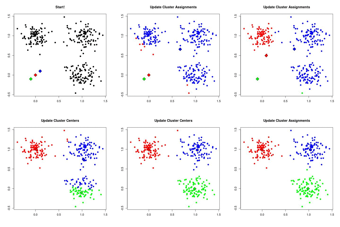
Here is an animated gif illustration of the k-means algorithm as it runs on the sample dataset used throughout this slecture. Deliberately poor starting locations of the cluster centers were chosen so that the algorithm would take several step to converge.

Figure 4

• A priori knowledge of the number of clusters is required
• K-means is sensitive to the starting location of the K clusters
• At each step, the distances between each data point and every cluster center must be computed, which can be slow for large data sets
• K-means uses the Euclidean distance as its measure of dissimilarity, which may be inappropriate for many data sets. A more general dissimilarity measure may be used, which results in the K-medoids algorithm. However, one must take care that step 3 can still be easily evaluated.

[1] Pattern Recognition and Machine Learning, 2006, by Christopher M. Bishop

Questions and comments

If you have any questions, comments, etc. please post them on this page.

Back to ECE662, Spring 2014