Discrete-time Fourier transform (DTFT) of a sampled cosine
A slecture by ECE student Yijun Han
Partly based on the ECE438 Fall 2014 lecture material of Prof. Mireille Boutin.
Contents
[hide]outline
- Introduction
- Sampling rate above Nyquist rate
- Sampling rate below Nyquist rate
- Conclusion
- References
Introduction
Consider a CT cosine signal (a pure frequency), and sample that signal with a rate above or below Nyquist rate. In this slecture, I will talk about how does the discrete-time Fourier transform of the sampling of this signal look like. Suppose the cosine signal is $ x(t)=cos(2\pi 440 t) $.
Sampling rate above Nyquist rate
The Nyquist sampling rate $ f_s=2f_M=880 $,so we pick a sample frequency 1000 which is above the Nyquist rate.
$ \begin{align} \\ x_1[n] & =x(\frac{n}{1000}) \\ & =cos(\frac{2\pi440 n}{1000}) \\ & =\frac{1}{2}(e^{\frac{j2\pi440 n}{1000}}+e^{\frac{-j2\pi440 n}{1000}})\\ \end{align} $
Since $ \frac{2\pi 440}{1000} $ is between $ -\pi $ and $ \pi $, so for $ \omega \isin [-\pi,\pi] $
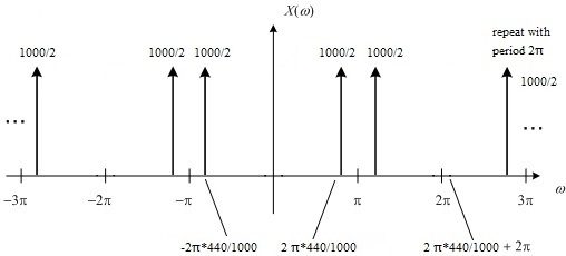
$ \begin{align} \\ \mathcal{X}_1(\omega) & =\frac{1}{2}[2\pi\delta(\omega-2\pi\frac{440}{1000})+2\pi\delta(\omega+2\pi\frac{440}{1000})] \\ & = \frac{1000}{2}[\delta(\frac{1000}{2\pi}\omega-440)+\delta(\frac{1000}{2\pi}\omega+440)] \end{align} $
For all w,
$ \mathcal{X}_1(\omega) = rep_{2\pi}{\frac{1000}{2}[\delta(\frac{1000}{2\pi}\omega-440)+\delta(\frac{1000}{2\pi}\omega+440)]} $
The graph of $ \mathcal{X}_1(\omega) $ is
Sampling rate below Nyquist rate
we pick a sample frequency 800 which is below the Nyquist rate.
$ \begin{align} \\ x_2[n] & =x(\frac{n}{800}) \\ & =cos(\frac{2\pi440 n}{800}) \\ & =cos(\frac{2\pi440 n}{800}-2\pi n) \\ & =cos(2\pi n \frac{-360}{800}) \\ & =cos(\frac{2\pi360 n}{800}) \\ & =\frac{1}{2}(e^{\frac{j2\pi360*n}{800}}+e^{\frac{-j2\pi360*n}{800}})\\ \end{align} $
Since $ \frac{2\pi*360}{800} $ is between $ -\pi $ and $ \pi $, so for $ \omega \isin [-\pi,\pi] $
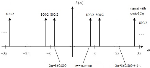
$ \begin{align} \\ \mathcal{X}_2(\omega) & =\frac{1}{2}[2\pi\delta(\omega-2\pi\frac{360}{800})+2\pi\delta(\omega+2\pi\frac{360}{800})] \\ & = \frac{800}{2}[\delta(\frac{800}{2\pi}\omega-360)+\delta(\frac{800}{2\pi}\omega+360)] \end{align} $
For all w,
$ \mathcal{X}_2(\omega) = rep_{2\pi}{\frac{800}{2}[\delta(\frac{800}{2\pi}\omega-360)+\delta(\frac{800}{2\pi}\omega+360)]} $
The graph of $ \mathcal{X}_2(\omega) $ is
Conclusion
The discrete Fourier transform of a sampled cosine signal with sample frequency f has the following properties:
compared with the CTFT of cosine signal
if f is above the Nyquist rate
1. $ \mathcal{X}(\omega) $ is a rep with period $ 2\pi $.
2. $ \mathcal{X}(\omega) $ re-scales by $ \frac{2\pi}{f} $.
3. $ \mathcal{X}(\omega) $ has amplitude of f.
if f is below the Nyquist rate
1. $ \mathcal{X}(\omega) $ is a rep with period $ 2\pi $.
2. $ \mathcal{X}(\omega) $ re-scales by $ \frac{2\pi(f-f_0)}{f} $.
3. $ \mathcal{X}(\omega) $ has amplitude of f.
References
[1].Mireille Boutin, "ECE438 Digital Signal Processing with Applications," Purdue University August 26,2009
[2].Steve Eddins,"Discrete-time Fourier transform (DTFT)," Matlab Central December 31, 2009
Questions and comments
If you have any questions, comments, etc. please post them on this page.


