Introduction to Maximum Likelihood Estimation

A slecture by Wen Yi

In statistics, maximum-likelihood estimation (MLE) is a method of estimating the parameters of a statistical model. When applied to a data set and given a statistical model, maximum-likelihood estimation provides estimates for the model's parameters. In maximum likelihood estimation, we search over all possible sets of parameter values for a specified model to find the set of values for which the observed sample was most likely. That is, we find the set of parameter values that, given a model, were most likely to have given us the data that we have in hand.

2. Basic method

Suppose there is a sample of n independent and identically distributed observations from a distribution with an unknown probability density function. We can say that the function belongs to a certain family of distributions , where θ is a vector of parameters for this family, so that so that . The value is unknown and is referred to as the true value of the parameter. So, using MLE, we want to find an estimator which would be as close to the true value as possible.

To use the method of maximum likelihood, one first specifies the joint density function for all observations. For an independent and identically distributed sample, this joint density function is：

As each sample x_i is independent with each other, the likelihood of θ with the observation of samples x_1,x_2,…,x_n can be defined as:

In practice, it’s more convenient to take ln for the both sides, called log-likelihhod. Then the formula becomes:

Then, for a fixed set of samples, to maximize the likelihood of θ, we should choose the data that satisfied: <span style="line-height: 1.5em;" />

To find the maximum of lnL(θ;x_1,x_2,…,x_N ), we take the derivative of θ on it and find theθ value that make the derivation equals to 0.

To check our result we should garentee that the second derivative of θ on lnL(θ;x_1,x_2,…,x_n ) is negative.

3. Practice considerations

3.1 Log-likelihood

Just as mentioned above, to make life a little easier, we can work with the natural log of likelihoods rather than the likelihoods themselves. The main reason for this is, computational rather than theoretical. If you multiply lots of very small numbers together (say all less than 0.0001) then you will very quickly end up with a number that is too small to be represented by any calculator or computer as different from zero. This situation will often occur in calculating likelihoods, when we are often multiplying the probabilities of lots of rare but independent events together to calculate the joint probability.

With log-likelihoods, we simply add them together rather than multiply them (log-likelihoods will always be negative, and will just get larger (more negative) rather than approaching 0).

So, log-likelihoods are conceptually no different to normal likelihoods. When we optimize the log-likelihood, with respect to the model parameters, we also optimize the likelihood with respect to the same parameters, for there is a one-to-one (monotonic) relationship between numbers and their logs.

3.2 Removing the constant

For example the likelihood function for the binomial distribution is:

In the context of MLE, we noted that the values representing the data will be fixed: these are n and k. In this case, the binomial 'co-efficient' depends only upon these constants. Because it does not depend on the value of the parameter p we can essentially ignore this first term. This is because any value for p which maximizes the above quantity will also maximize.

This means that the likelihood will have no meaningful scale in and of itself. This is not usually important, however, for as we shall see, we are generally interested not in the absolute value of the likelihood but rather in the ratio between two likelihoods - in the context of a likelihood ratio test.

We may often want to ignore the parts of the likelihood that do not depend upon the parameters in order to reduce the computational intensity of some problems. Even in the simple case of a binomial distribution, if the number of trials becomes very large, the calculation of the factorials can become infeasible.

3.3 Numerical MLE

Sometimes we cannot write an equation that can be differentiated to find the MLE parameter estimates. This is especially likely if the model is complex and involves many parameters and/or complex probability functions. (e.g. the normal mixture probability distribution)

In this scenario, it is also typically not feasible to evaluate the likelihood at all points, or even a reasonable number of points. In the parameter space of the problem in the coin toss example, the parameter space was only one-dimensional (i.e. only one parameter) and ranged between 0 and 1. Nonetheless, because p can theoretically take any value between 0 and 1, the MLE will always be an approximation (albeit an incredibly accurate one) if we just evaluate the likelihood for a finite number of parameter values. For example, we chose to evaluate the likelihood at steps of 0.02. But we could have chosen steps of 0.01, of 0.001, of 0.000000001, etc. In theory and practice, one has to set a minimum tolerance by which you are happy for your estimates to be out. This is why computers are essential for these types of problems: they can tabulate lots and lots of values very quickly and therefore achieve a much finer resolution.

4. Some basic examples

4.1 Poisson Distribution

For Poisson distribution the expression of probability is:

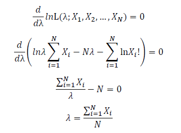
Let X_1,X_2,…,X_N be the Independent and identically distributed (iid) Poisson random variables. Then, we will have a joint frequency function that is the product of marginal frequency functions. The log likelihood of Poisson distribution thus should be:

Take the derivative of λ on it and find theλ value that make the derivation equals to 0.

Thus, the ML estimation for Poisson distribution should be:

4.2 Exponential distribution

For exponential distribution the expression of probability is:

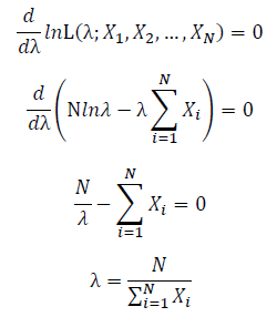
Let X_1,X_2,…,X_N be the Independent and identically distributed (iid) exponential random variables. As P(X=x)=0 when x<0, no samples can sit in x<0 region. Thus, for all X_1,X_2,…,X_N, we can only focus on the x≥0 part. Then, we will have a joint frequency function that is the product of marginal frequency functions. The log likelihood of exponential distribution thus should be:

Take the derivative of λ on it and find theλ value that make the derivation equals to 0.

Thus, the ML estimation for exponential distribution should be:

4.3 Gaussian distribution

For Gaussian distribution the expression of probability is:

Let X_1,X_2,…,X_N be the Independent and identically distributed (iid) Gaussian random variables. Then, we will have a joint frequency function that is the product of marginal frequency functions. The log likelihood of Gaussian distribution thus should be:

Take the derivative of μ,Σ on it and find the μ,Σ value that make the derivation equals to 0.

Thus, the ML estimation for Gaussian distribution should be:

5. Some advanced examples

5.1 Expression of Estimated Parameters

The above estimation all base on the assumption that the distribution to be estimated follows the distribution of a single function, but how about the estimation of the mixture of functions?

To simplify the problem, we only talk about Gaussian Mixture Model (GMM) here. Using the same method, it’s easy to extend it to other kind of mixture model and the mixture between different models.

To start with, we should know that if we set the number of Gaussian function to be used in the GMM estimation flexible, we will find out that the number of Gaussian function will never reach a best solution, as adding more Gaussian functions into the estimation will subsequently improve the accuracy anyway. As calculating how many Gaussian function is include in GMM is a clustering problem. We assume to know the number of Gaussian function in GMM as k here.

As this distribution is a mixture of Gaussian, the expression of probability is:

α_j is the weight of Gaussian function g_j (x).

Thus, the parameters to be estimated are:

Let X_1,X_2,…,X_N be the Independent and identically distributed (iid) Gaussian Mixture Model (GMM) random variables.

Following Bayes rule, the responsibility that a mixture component takes for explaining an observation X_i is:

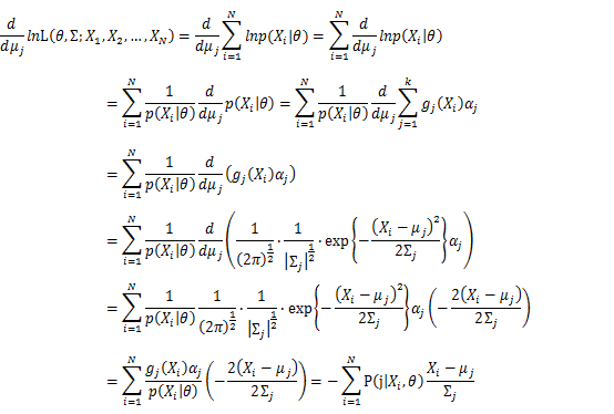
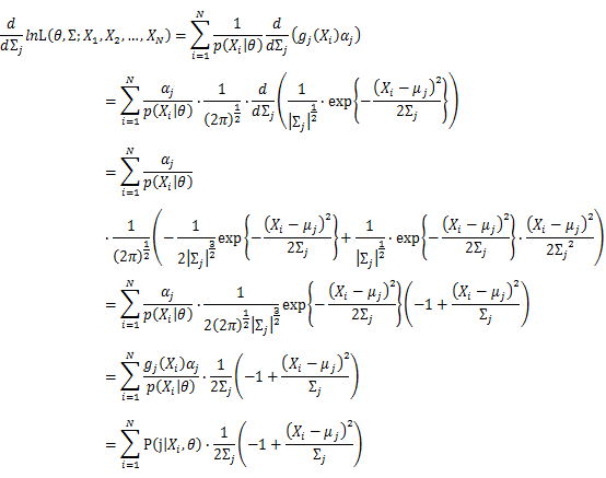
Then, we will have a joint frequency function that is the product of marginal frequency functions. The log likelihood of Gaussian Mixture Model distribution thus should be:

Take the derivative of μ_j,Σ_j on it and find the μ_j,Σ_j value that make the derivation equals to 0.

The α_j is subject to

Basic optimization theories show that α_j is optimized by:

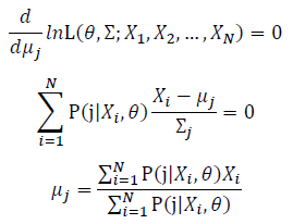
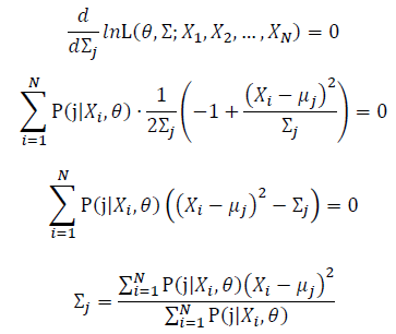
Thus, the ML estimation for Gaussian Mixture Model distribution should be:

5.2 Practical Implementation

Now we can observe that, as the Gaussian Mixture Model with K Gaussian functions have 3K parameters, to find the best vector of parameters set, θ, is to find the optimized parameters in 3K dimension space. As the Gaussian Mixture Model include more Gaussian functions, the complexity of computing the best θ will go incrediblily high. Also, we can see that all the expressions of μ, Σ and α include themselves directly or indirectly, it’s implossible to get the value of the parameters within one time calculation.

Now it’s time to introduce a method for finding maximum likelihood with large number of latent variables (parameters), Expectation–maximization (EM) algorithm.

In statistics, an expectation–maximization (EM) algorithm is an iterative method for finding maximum likelihood estimates of parameters in statistical models, where the model depends on unobserved latent variables (the parameters). The EM iteration alternates between performing an expectation (E) step, which creates a function for the expectation of the log-likelihood evaluated using the current estimate for the parameters, and a maximization (M) step, which computes parameters maximizing the expected log-likelihood found on the E step. These parameter-estimates are then used to determine the distribution of the latent variables in the next E step.

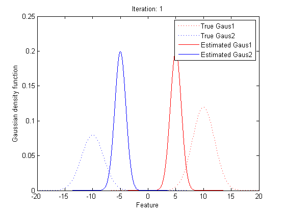
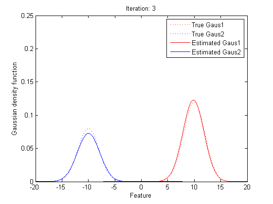
In short words, to get the best θ for our maximum likelihood, firstly, for the expectation step, we should evaluate the weight of each cluster with the current parameters. Then, for the maximization step, we re-estimate parameters using the existing weight.

By repeating these calculation process for several times, the parameters will approach the value for the maximum likelihood.