Bayes Parameter Estimation (BPE) tutorial

                                                A slecture by ECE student Haiguang Wen

                       Partially based on the ECE662 lecture material of Prof. Mireille Boutin.

 1. What will you learn from this slecture?

• Basic knowledge of Bayes parameter estimation
• An example to illustrate the concept and properties of BPE
• The effect of sample size on the posterior
• The effect of prior on the posterior

2. Introduction

Bayes parameter estimation (BPE) is a widely used technique for estimating the probability density function of random variables with unknown parameters. Suppose that we have an observable random variable X for an experiment and its distribution depends on unknown parameter θ taking values in a parameter space Θ. The probability density function of X for a given value of θ is denoted by p(x|θ ). It should be noted that the random variable X and the parameter θ can be vector-valued. Now we obtain a set of independent observations or samples S = {x₁,x₂,...,x_n} from an experiment. Our goal is to compute p(x|S) which is as close as we can come to obtain the unknown p(x), the probability density function of X.

In Bayes parameter estimation, the parameter θ is viewed as a random variable or random vector following the distribution p(θ ). Then the probability density function of X given a set of observations S can be estimated by

                                                       $ \begin{align} p(x|S)&= \int p(x,\theta |S) d\theta \\ &= \int p(x|\theta,S)p(\theta|S)d\theta \\ &= \int p(x|\theta)p(\theta|S)d\theta \end{align} $                                                       (1)

So if we know the form of p(x|θ) with unknown parameter vector θ, then we need to estimate the weight p(θ |S), often called posterior, so as to obtain p(x|S) using Eq. (1). Based on Bayes Theorem, the posterior can be written as

                                                        $ p(\theta|S) = \frac{p(S|\theta)p(\theta)}{\int p(S|\theta)p(\theta)d\theta} $                                                                 (2)

where p(θ) is called prior distribution or simply prior, and p(S|θ) is called likelihood function [1]. A prior is intended to reflect our knowledge of the parameter before we gather data and the posterior is an updated distribution after obtaining the information from data.

3. Estimate posterior 

In this section, let’s start with a tossing coin example [2]. Let S = {x₁,x₂,...,x_n} be a set of coin flipping observations, where x_i = 1 denotes 'Head' and x_i = 0 denotes 'Tail'. Assume the coin is weighted and our goal is to estimate parameter θ , the probability of 'Head'. Assume that we flipped a coin 20 times yesterday, but we did not remember how many times the ’Head’ was observed. What we know is that the probability of 'Head' is around 1/4, but this probability is uncertain since we only did 20 trails and we did not remember the number of 'Heads'. With this prior information, we decide to do this experiment today so as to estimate the parameter θ .

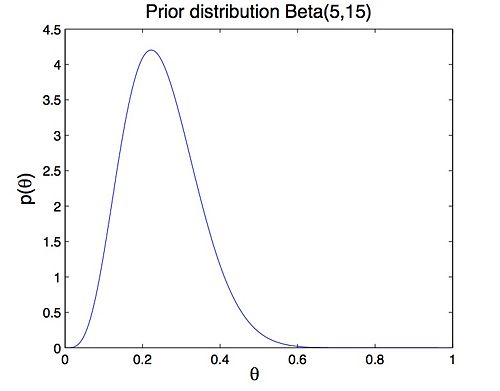
A prior represents our previous knowledge or belief about parameter θ. Based on our memories from yesterday, assume that the prior of θ follows Beta distribution Beta(5, 15) (Figure 1).

                                                             $ \text{Beta}(5,15) = \frac{\theta^{4}(1-\theta)^{14}}{\int\theta^{4}(1-\theta)^{14}d\theta} $                                                    (3) 

                                                           Figure 1: Prior distribution Beta(5, 15)

Today we flipped the same coin n times and y 'Heads' were observed. Then we compute the posterior with today’s data. Consider Eq. (2), the posterior is written as

                                                          $ \begin{align} p(\theta|S) &= \frac{p(S|\theta)p(\theta)}{\int p(S|\theta)p(\theta)d\theta}\\ &= \text{const}\times \theta^{y}(1-\theta)^{n-y}\theta^4(1-\theta)^{14}\\ &=\text{const}\times \theta^{y+4}(1-\theta)^{n-y+14}\\ &=\text{Beta}(y+5, \;n-y+15) \end{align} $                                (4)

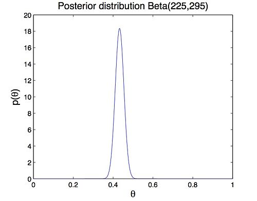
Assume that we did 500 trials and 'Head' appeared 220 times, the posterior is Beta(225,295) (Figure 2). It can be noted that the posterior and prior distribution have the same form. This kind of prior distribution is called conjugate prior. The Beta distribution is conjugate to the binomial distribution which gives the likelihood of i.i.d Bernoulli trials.

                                                      Figure 2: posterior distribution Beta(225, 295)

As we can see, the conjugate prior successfully includes previous information, or our belief of parameter θ into the posterior. So our knowledge about the parameter is updated with today’s data, and the posterior obtained today can be used as prior for tomorrow’s estimation. This reveals an important property of Bayes parameter estimation, that the Bayes estimator is based on cumulative information or knowledge of unknown parameters, from past and present.

4. Estimate density function of random variable

After we obtain the posterior, then we can estimate the probability density function of random variable X. Consider Eq. (1), the density function can be expressed as

                                            $ \begin{align} p(x|S) &= \int p(x|\theta)p(\theta|S)d\theta\\ &=\text{const}\int \theta^x(1-\theta)^{1-x}\theta^{y+4}(1-\theta)^{n-y+14}d\theta\\ &= \left\lbrace \begin{array}{ll} \frac{y+5}{n+20} & x=1\\ \\ \frac{n-y+15}{n+20} & x=0 \end{array} \right. \end{align} $                                    (5)

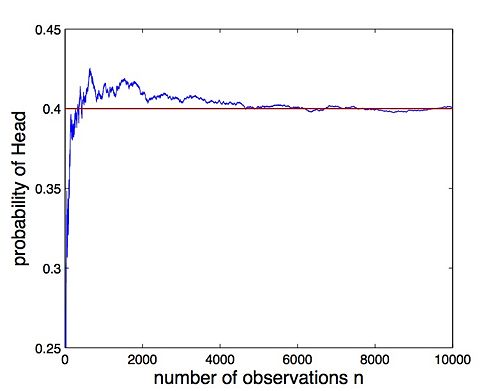
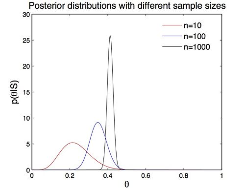
It suggests that the prior Beta(5,15) actually is equivalent to adding 20 Bernoulli observations to the data, 5 Heads and 15 Tails. This means the posterior summarizes all our knowledge about the parameter x, and the prior does affect the estimate of the density of random variable X. However, as we do more and more coin flipping trials (i.e. n is getting larger), the density function p(x|S) will almost surely converge to the underlying distribution (Figure 3), which means the prior becomes less important. Figure 4 illustrates that as n is getting larger, the posterior becomes sharper. In our experiment, when n = 10000, the posterior has sharply peak at θ = 0.4. In this case, the prior (said around 1/4) has little effect on posterior and we have strong belief to say that the probability of ’Head’ is around 0.4.

                                                    Figure 3: the probability of 'Head' varies with sample size 

                                             Figure 4: posterior distribution derived from different sample sizes

5. Gaussian model

The Bernoulli distribution discussed above is a discrete example, here we will illustrate a continuous example, a Gaussian random variable X [3]. Assume S = {x₁,x₂,...,x_n} is a set of independent observations of a Gaussian random variable X ∼ N(μ,σ²) with unknown mean μ. Here we use a conjugate prior $ p(\mu) \sim N(\mu_0,\sigma_0^2) $. Then the posterior can be computed by

                                         $ \begin{align} p(\mu|S) &= \frac{p(S|\theta)p(\theta)}{\int p(S|\theta)p(\theta)d\theta}\\ &= \text{const}\times\left[\prod_{i=1}^n \exp\{-\frac{(x_i-\mu)^2}{2\sigma^2}\}\right]\times\exp\{-\frac{(\mu-\mu_0)^2}{2\sigma_0^2}\}\\ &= \text{const}\times \exp\{-\frac{(\mu-\mu_n)^2}{2\sigma_n^2}\}\\ &= N(\mu_n, \sigma_n^2) \end{align} $                     (6)

So the posterior also follows Gaussian distribution $ N(\mu_n,\sigma_n^2) $, where μn and $ \sigma_n^2 $ is defined by

                                                   $ \begin{align} \mu_n &= \left(\frac{n\sigma_0^2}{n\sigma_0^2+\sigma^2}\right)\bar{x}+\frac{\sigma^2}{n\sigma_0^2+\sigma^2}\mu_0\\ \sigma_n^2 &= \frac{\sigma_0^2\sigma^2}{n\sigma_0^2+\sigma^2} \end{align} $                                                       (7)

Consider Eq. (1), we have the estimated density of random variable X.

                                             $ \begin{align} p(x|S) &= \int p(x|\mu)p(\mu|S)d\mu\\ &=\text{const}\times\int \exp \left\lbrace-\frac{(x-\mu)^2}{2\sigma^2}\right\rbrace \exp \left\lbrace-\frac{(\mu-\mu_n)^2}{2\sigma_n^2}\right\rbrace d\mu\\ &=\text{const}\times\exp \left\lbrace-\frac{(x-\mu_n)^2}{2(\sigma^2+\sigma_n^2)}\right\rbrace\\ &= N(\mu_n,\sigma^2+\sigma_n^2) \end{align} $                   (8)

5.1 Different sample sizes with fixed prior

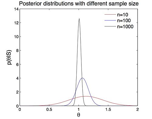
Assume that the true mean of the distribution p(x) is μ = 1 with standard deviation σ = 1. And the prior distribution is set to p(θ) ∼ N(0.5,0.5). Then we estimate the posterior with different sample sizes (i.e. different number of observations n).

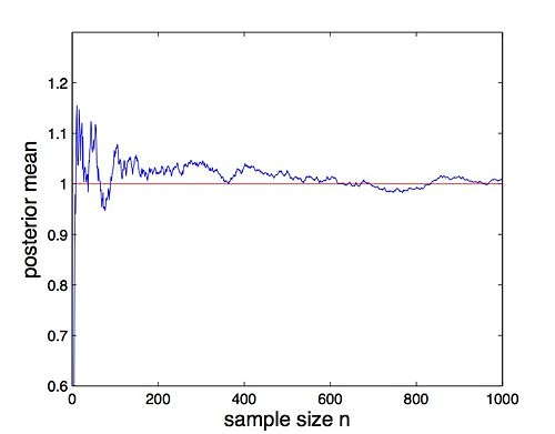
Similar to the coin flipping experiment, the posterior becomes more and more sharply peaked and centers at around μ = 1 as the number of observations increases (Figure 5). Figure 6 suggests that the mean converges to 1 as n → ∞. However, when the sample size is small (e.g. n = 50), the posterior is greatly affected and biased by the prior.

                                     Figure 5: posteriors derived from different sample size (Gaussian model)           

                                           Figure 6: posterior mean varies with sample size n (Gaussian model)

5.2 Different priors with fixed sample size

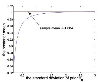
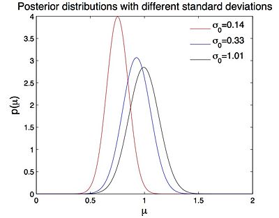
Last section tells us that the prior affects the posterior if present data is limited. Here we consider priors $ p(\mu) \sim N(0.5,\sigma_0^2) $ with different standard deviations σ₀.

Consider Eq.(7), we note that if the posterior distribution becomes, which suggests that the mean of the posterior is the empirical sample mean. Figure 7 shows that as σ₀ is getting larger, the prior becomes more 'uniform' over (−∞,∞). That the prior is ’uniform’ means the parameter takes any value in (−∞,∞) with identical probability. And this means that we can not provide any previous information about the parameter. So if σ0 is very big, the prior has little effect on posterior. The experimental result (Figure 8) also suggests the same issue: the posterior mean become closer to sample mean as σ0 is getting larger, i.e. the prior contributes little to posterior if σ0 is very big.

                                              Figure 7: Gaussian prior N(0.5, \sigma) with different standard deviations

                              Figure 8: (a) posterior mean varies with the standard deviation of prior                                                                                (b) posteriors derived from three priors with different standard deviations

Combining section 5.1 and 5.2, we suggest that if sample size is small and prior informative is limited, then we need to select a larger σ₀ for conjugate prior so that the prior would not greatly affect and bias the posterior. For multivariate Gaussian model, please refer to Multivariate Gaussian.

6. Summary of BPE

Bayes parameter estimation is a very useful technique to estimate the probability density of random variables or vectors, which in turn is used for decision making or future inference. We can summarize BPE as

1.  Treat the unknown parameters as random variables
2. Assume a prior distribution for the unknown parameters
3. Update the distribution of the parameter based on data
4. Finally compute p(x | S)
   
   

7. Further Study

This slecture only introduces the basic knowledge about BPE. In practice, there are some important issues that need to be considered.

• Set up a appropriate prior. Since the prior distribution is a key part of Bayes estimator and inappropriate choices for priors can lead to incorrect inferences. According to our knowledge to a parameter, the prior usually can be classified to two classes: informative prior and noninformative [4]. 
• Calculate p(x | S) with two integrals. Usually, the required integrations will not be feasible analytically and, thus, efficient approximation strategies are required. There are many different types of numerical approximation algorithms in Bayesian inference, such as Approximate Bayesian Computation (ABC),Laplace Approximation and Markov chain Monte Carlo (MCMC).

Reference

[1] Mireille Boutin, "ECE662: Statistical Pattern Recognition and Decision Making Processes," Purdue University, Spring 2014.
[2] Carlin, Bradley P., and Thomas A. Louis. ”Bayes and empirical Bayes methods for data analysis.” Statistics and Computing 7.2 (1997): 153-154.
[3] Box, George EP, and George C. Tiao. Bayesian inference in statistical analysis. Vol. 40. John Wiley & Sons, 2011.
[4] Gelman, Andrew. ”Prior distribution.” Encyclopedia of environmetrics (2002).

Questions and comments

If you have any questions, comments, etc. please post them on this page.

Categories: ECE662 | Bayes' Theorem |Probability | Bayes' Rule | Bayes' Classifier | Slecture | ECE662Spring2014Boutin | ECE | Pattern recognition