Introduction
The PCA, or Principal Component Analysis is used to find a lower dimensional subspace that best represents the data according to the squared-error criterion function defined as
$ J_0(\vec{x_0}) = \sum_{k=1}^{n}\| \vec{x_0} - \vec{x_k}\|^2 $
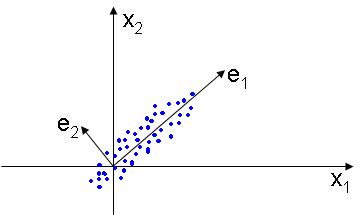
This method works by placing the basis of the new linear subspace in the directions that the data varies most, in other words, each dimension of the new space is selected in order to account for most of the variation of the data. The figure below illustrates this idea:
Another way to interpret this transformation is to say that the data points are projected in a new feature space where the new features are uncorrelated.
Computing the PCA
In order to compute the basis of the new subspace that best represents the data, the PCA diagonalizes the maximum likelihood estimate of the covariance matrix
$ C=\frac{1}{n} \sum_{i=1}^{n} \vec{x_i}\vec{x_i}^T $
by solving the eigenvalue equation
$ C\vec{e} = \lambda \vec{e} $
The solutions to these equations are eigenvalues $ \lambda_1 \geqslant \lambda_2 \geqslant \cdots \geqslant \lambda_k \geqslant \cdots \geqslant \lambda_m $. Often only $ k \leqslant m $ eigenvalues will have a nonzero value, meaning that the inherent dimensionality of the data is $ k $, being $ n-k $ dimensions noise in the data.
In order to represent the data in the k dimensional space we first construct the matrix $ E=[\vec{e_1} \vec{e_2} \cdots \vec{e_k}] $. The projection to the new k-dimensional subspace is done by the following linear transformation:
$ \vec{x}^{'} = E^T\vec{x} $
Dimensionality Reduction
By selecting the eigenvectors corresponding to the k largest eigenvalues from the eigenvalue equation, we project the data in a k- dimensional subspace that best represents the data variability in each dimension. In some datasets, many of the eigenvalues $ \lambda_i $ will be zero. This means that the intrinsic dimensionality of the data is smaller than the dimensionality of the input samples.
Limitations
Nonlinear data embedding: The PCA method finds a low-dimensional subspace and embeds the data points in that subspace in a way that best preserves the variance of the input space (original high-dimensional space). If the input data points are embedded in nonlinear structures (nonlinear manifolds), those structures would not be visible to the PCA, and the method will fail in detecting the data's true degrees of freedom. Methods that explore nonlinear manifolds should be used in those situations. These methods include Isomap, Laplacian Eigenmaps, LLE, among others.
Computational Efficiency: The solution to the eigensystem stated above may incur in large computational cost, for high dimensional data, since the cost of the eigendecomposition is $ O(m^3) $. This may be prohibitive for many applications. The solutions to the complexity problem are based on the observation that only the eigenvectors corresponding to the largest k eigenvalues are of practical interest. Therefore, numerical approximations to the desirable k eigenvectors without performing the whole eigendecomposition of a $ m \times m $ matrix are of extreme importance. Several methods have been proposed to overcome the high computational cost problem. Very common ones are the ones based on the Nystrom Method.
References
- Wikipedia[1]
- "Pattern Classification" by Duda, Hart, and Stork_OldKiwi
- "Approximating a Gram Matrix for Improved Kernel-Based Learning", P. Drineas and M. Mahoney in Proceedings of the 18th Annual Conference on Learning Theory, 2005.


