Parametric Methods
Two applications:
- Parametric Density Estimation: Using sample data, we estimate probabilities $ P(\omega_i) $, $ p(\vec{X}|\omega_i) \forall i $ etc using estimation methods like [MLE] and [BPE]. Then from these estimated probabilities (and not true probabilities, which are unknown; only their parametric form was known) we can use Bayes classification rule to build a classifier.
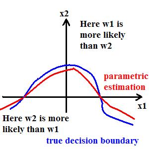
- Parametric Classifiers_OldKiwi: We find parametric decision boundaries to approximate true decision boundaries between classes. This is very different approach from approximating the probabilities with their estimates, as in previous method.
Example:

True decision boundary: $ \{\vec{X}|P(\omega_1|\vec{X})-P(\omega_2|\vec{X})=0\} $ can be approximated by $ \{\vec{X}|g(\vec{X})=0\} $. Note that 'g' is not an estimate of the difference in probabilities as in true decision boundary, but it is just an approximate parametric form for the true decision boundary. Choice of 'g' depends on whether it is analytic, and hence easy to handle computationally.
E.g. 'g' can be a degree-2 polynomial, or it can be a degree-1 polynomial (resulting in a linear classifier).
If 'g' is linear, it can be written as $ g(\vec{X})=\vec{V}.\vec{X}+V_0=(\vec{V},V_0).(\vec{X},1) $ or $ g(1,\vec{X})=\vec{c}.(1,\vec{X}) $.
- Extension of Feature Space**
This trick justifies the importance of studying linear classifiers even though they do not occur so often in practice directly. Actually, many non-linear classifiers can be seen as linear.
Example 1: Consider g to be a polynomial parametric form of a classifier in $ \mathbb{R}^2 $.
$ g(x,y)=c_0+c_1x+c_2y+c_3xy+c_4{x}^2+c_5{y}^2 $
.. |g_tilde_from_5_1| image:: tex
- alt: tex: \tilde{g}:\mathbb{R}^5 \to \mathbb{R}
.. |g_tilde_def1| image:: tex
- alt: tex: \tilde{g}(u_1,u_2,u_3,u_4,u_5)=c_0+c_1u_1+c_2u_2+c_3u_3+c_4u_4+c_5u_5
Here g is not a linear classifier in |R_squared1|. Let us define |g_tilde_from_5_1|
|g_tilde_def1|
.. |change_var1| image:: tex
- alt: tex: u_1=x; u_2=y; u_3=xy; u_4={x}^2; u_5={y}^2
where |change_var1|. Here we have defined a parametric from of the classifier in extended feature space. This form is linear. Hence "Decision boundary defined by 'g' is linear in extended feature space."
Example 2: Consider another polynomial,
|circle_ex|
.. |circle_ex| image:: tex
- alt: tex: g(x)={x}^2+{y}^2-2{y}
= {x}^2+{(y-1)}^2 -1 This is a circle centred at (0,1):
.. image:: Circle.jpg
This non-linear function can be transformed into linear function in extended feature space like below.
|jinha_linear_circle|
.. |jinha_linear_circle| image:: tex
- alt: tex: \{ (x, y, x^2, y^2) \mid (0, -2, 1, 1) \cdot (x, y, x^2, y^2) = 0 \}
.. image:: lec9_embedd.bmp
Example 3: 1D example
.. image:: Jinha_1D_Example01.jpg
As we can see from above figure, decision boundary is not linear ( region is not connected). From this, we can construct an extended [feature vector] space.
|jinha_xx2|
.. |jinha_xx2| image:: tex
- alt: tex: x \rightarrow (x, x^2) \in R^2
.. image:: Jinha_1D_Example02.jpg
This red line (which is a hyperplane in this case) can separate these two classes. This can be expressed as below mathematical form.
|jinha_pp2|
.. |jinha_pp2| image:: tex
- alt: tex: p(x \mid w_1) \rightarrow p(x, x^2 \mid w_1)
.. |g_vc| image:: tex
- alt: tex: \vec{g}
.. |g_vec_eq| image:: tex
- alt: tex: g(\vec{X})=\sum_{i=1}^{n}{\lambda}_{i}{e}^{{c}_{i}\vec{x}}
.. |g_x| image:: tex
- alt: tex: g(\vec{x})
- Taylor Series** If true |g_vc| is analytic
e.g |g_vec_eq|
then, |g_x| = Taylor Series --> infinite polynomial in powers
because we can approximate with Taylor plynomial of degree n (i.e as n get higher, approximatino gets better)
.. image:: poly2.gif
However, there are issues on this approach. It gets complex with the increase of the dimension of the [feature vector].
If |jinha_x|
.. |jinha_x| image:: tex
- alt: tex: \vec{x} = (x_1, x_2, \cdots, x_d)
A degree 2 polynomial in |jinha_x| has |jinha_dim2poly| monomials
.. |jinha_dim2poly| image:: tex
- alt: tex: \frac{1}{2} (d+1) (d+2) \approx d^2
A degree n polynomial in |jinha_x| has |jinha_dn| monomials.
.. |jinha_dn| image:: tex
- alt: tex: \approx d^n
- How to find decision hyperplane given training data**
In the best of all cases, data is "linearly separable", meaning there exists a vector c such that for all y training data: c * y > 0 if y belongs to class w1. (where * is a dot product) c * y < 0 of u belongs to class w2.
- Trick:** replace all y's in the training data belonging to class w2 by -y, then look for vector c such that
c * y > 0 for all y.
Example: 1D feature space
x->(1,x)=:y
.. image:: Lecture9_1D_yi_-yi.JPG
First component is +1 for all of class 1 training data
First component is -1 for all of class 2 training data
.. image:: Lecture9_1D_yi_-yi_2.JPG
Observe: c is not unique
To make |vec_c| unique, introduce 'margin' b>0 and ask that c be the minimum length vector such that |khh0|, for all i
.. |khh0| image:: tex
- alt: tex: \vec{c} \cdot y_{i} \geq b
.. |vec_c| image:: tex
- alt: tex: \vec{c}
- Geometric Interpretation of margin**
If |khh1|, then |vec_c| belons to hyperplane with normal vector |y_io| which is at distance |b_over_y_io| from the origin.
.. |khh1| image:: tex
- alt: tex: \vec{c} \cdot y_{i} = b
.. |y_io| image:: tex
- alt: tex: y_{i0}
.. |b_over_y_io| image:: tex
- alt: tex: \displaystyle \frac{b} {\displaystyle ||y_{i0} ||}
|khh0|, for all i means that |vec_c| is always at least a distance |b_over_y_io| from the origin for all i
In general, it is impossible to satisfy |khh2|, for all i
.. |khh2| image:: tex
- alt: tex: \vec{c} \cdot y_{i} \geq 0
Perhaps, we could try to minimize number of mislassfied training samples
Let |khh5| -> Too hard to minimize.
.. |khh5| image:: tex
- alt: tex: J(\vec{c})=\{ y_{i} | \vec{c} \cdot y_{i} \leq 0 \}
- [Perceptron] Criterion function**
|khh6|
.. |khh6| image:: tex
- alt: tex: J_{p}(\vec{c})=\displaystyle \sum_{y_i, missclassified} (- \vec{c} \cdot y_{i} )
.. image:: lec9_percept.bmp
Measure how 'far away' you are from bias right. distance from |y_i| to hyperplane defined by |vec_c| is |khh3|
.. |y_i| image:: tex
- alt: tex: y_{i}
.. |khh3| image:: tex
- alt: tex: ||\vec{y_i} \cdot \frac{\vec{c}}{||\vec{c}||} ||=\frac{1}{|| \vec{c} ||} \vec{y_i} \cdot \vec{c}
Since |khh4| is proportional to distance from |y_i| to hyperplane
.. |khh4| image:: tex
- alt: tex: \vec{c} \cdot \vec{y}


