Text slecture - Rhea

Outline

1. Introduction
2. Definition of Downsampling
   
3. Derivation of DTFT of downsampled signal
   
4. Example
5. Conclusion
6. References

Introduction

This slecture provides definition of downsampling, derives DTFT  downsampled signal and demonstrates it in a frequency domain. Also, it explains process of decimation and why it needs a low-pass filter.

Definition of Downsampling

Downsampling is an operation which involves throwing away samples from discrete-time signal. Let  x[n] be a digital-time signal shown below:

GRAPH

 then y[n] will be produced by downsampling x [n]  by factor D = 3. So, y [n] = x[Dn].

GRAPH

As seen in above graph, y [n] is obtained by throwing away some samples from x [n]. So, y [n] is a downsampled signal from

x [n].

Derivation of DTFT of downsampled signal

Let x (t) be a continuous time signal. Then x₁ [n] = x (T₁n) and  x₂ [n] = x (T₂n). And ratio of sampling periods would be

D = T₂/T₁,   which is an integer greater than 1. From these equations we obtain realtionship between x₁ [n] and x₂ [n].

$ \begin{align} x_2 [n] = x(T_2 n) = x(DT_1 n) = x_1 [nD] \end{align} $

Below we derive Discrete-Time Fourier Transform of x₂ [n] in terms of DTFT of x₁ [n].

$ \begin{align} &\mathcal{X}_2(\omega)= \mathcal{F}(x_2 [n]) = \mathcal{F}(x_1 [Dn])\\ &= \sum_{n = -\infty}^\infty x_1[Dn] e^{-j \omega n} = \sum_{m = -\infty}^\infty x_1[m] e^{-j \omega {\frac{m}{D}}}\\ &= \sum_{n = -\infty}^\infty s_D[m]* x_1 [m] e^{-j \omega {\frac{m}{D}}}\\ \end{align} $

where

$ s_D [m]=\left\{ \begin{array}{ll} 1,& \text{ if } n \text{ is a multiple of } 4,\\ 0, & \text{ else}. \end{array}\right. = {\frac{1}{D}} \sum_{k = -\infty}^{D-1} e^{jk {\frac{2 \pi}{D} m}} $

$ \begin{align} &\mathcal{X}_2(\omega)= \sum_{m = -\infty}^\infty {\frac{1}{D}} \sum_{k = -\infty}^{D-1} e^{jk {\frac{2 \pi}{D} m}} x_1[m] e^{-j \omega {\frac{m}{D}}}\\ &= {\frac{1}{D}} \sum_{k = -\infty}^{D-1} \sum_{m = -\infty}^\infty x_1[m] e^{-jm ({\frac{\omega - 2 \pi k}{D}})} = \\ &= {\frac{1}{D}} \sum_{k = -\infty}^{D-1} \mathcal{X}_1 ({\frac{\omega - 2 \pi k}{D}}) \\ \end{align} $

Example

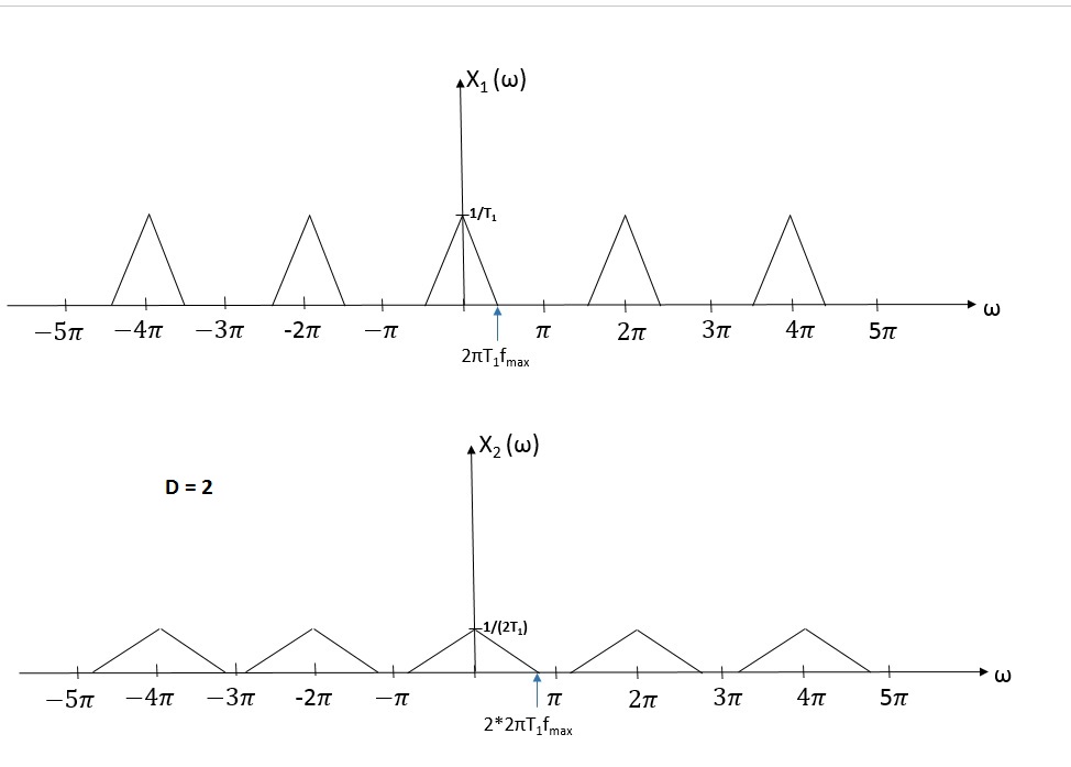
Let's take a look  at  an original signal X₁ (w) and  X₂ (w) which is obtained after downsampling X₁(w) by factor D = 2 in a frequency domain.

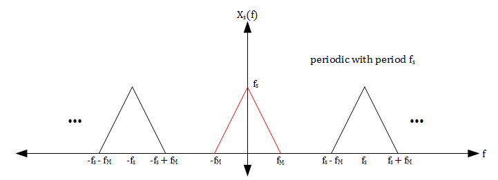
We would like to determine what X_s(f) looks like in order to find a way to reconstruct x(t).

Since we have sampled at a rate f_s > 2f_M, the following inequalities hold:

$ f_s > 2f_M \iff f_s - f_M > f_M \iff -f_s + f_M < f_M $.

Together, these inequalities, the graph of X(f), and the expression for X_s(f) in terms of X(f) imply that X_s(f) will have the spectrum shown in the figure below.

Notice that the spectrum of the ideal sampling of a signal is an amplitude scaled periodic repetition of the original spectrum. Since x(t) is bandlimited and we have sampled at a rate f_s > 2f_M, the periodic repetitions of X(f) do not overlap.

All the information needed to reconstruct X(f) can be found in the portion of X_s(f) that corresponds to X(f) (shown in red). Therefore we can use a simple lowpass filter with gain $ \tfrac{1}{f_s} $ and cutoff frequency $ \tfrac{f_s}{2} $ to recover X(f) from X_s(f).

$ X(f) = X_s(f)\left\{ \begin{array}{ll} \frac{1}{f_s}, & |f| \le \frac{f_s}{2}\\ 0, & \text{else} \end{array} \right. $

$ \iff x(t) = x_s(t)*\text{sinc}(f_st) $

$ \therefore $ We can perfectly reconstruct x(t) from x_s(t).

Example

Though the Nyquist theorem states that perfect reconstruction is possible if we satisfy the Nyquist condition (f_s > 2f_M), it is important to note that this condition is not necessary. The following example demonstrates how perfect reconstruction is sometimes possible even when undersampling.

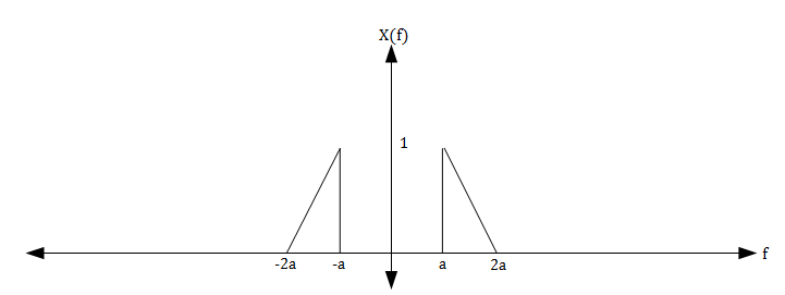
Let the signal x(t) have a spectrum X(f) as seen in the figure below.

The Nyquist condition states that we should sample at a rate f_s > 2(2a) = 4a. Instead, let us sample at f_s = 2a.

As before, we have $ x_s(t) = x(t)p_{\frac{1}{f_s}}(t) $ and $ X_s(f) = f_s\sum_{k = -\infty}^\infty X(f-kf_s) $

$ \implies X_s(f) = 2a\sum_{k = -\infty}^\infty X(f-2ka) $.

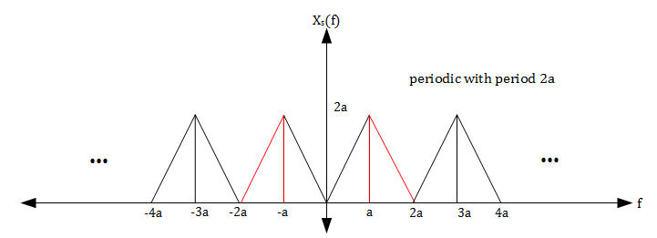
Therefore, X_s(f) will have the spectrum shown in the figure below.

Notice that there is no aliasing in X_s(f) even though f_s < 4a. In addition, the portion of X_s(f) that corresponds to X(f) (shown in red) can be recovered using a bandpass filter with gain $ \tfrac{1}{2a} $ and cutoff frequencies a and 2a.

Conclusion