Estimation Using Nearest Neighbor - Rhea

Introduction

In this slecture, basic principles of implementing nearest neighbor rule will be covered. The error related to the nearest neighbor rule will be discussed in detail including convergence, error rate, and error bound. Since the nearest neighbor rule relies on metric function between patterns, the properties of metrics will be studied in detail. Example of different metrics will be introduced with its characteristics. The representative of real application such as body posture recognition using Procrustes metric could be a good example to understand the nearest neighbor rule.----

Nearest Neighbor Basic Principle

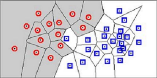
Let's consider a testing sample x. Based on labeled training sample $ D^n = x_{1},... ,x_{n}, $ the nearest neighbor technique will find the closest point x' to x. Then we assign the class of x' to x. This is how the classification based on the nearest neighbor rule is processed. Although this rule is very simple, it is also reasonable. The label $ \theta' $ used in the nearest neighbor is random variable which means $\theta' = w_{i}$ is same as a posteriori probability $P(w_{i}|x').$ If sample sizes are big enough, it could be assumed that x' is sufficiently close to x that $ P(w_{i}|x') = P(w_{i}|x). $ Using the nearest neighbor rule, we could get high accuracy classification if sample sizes are guaranteed. In other words, the nearest neighbor rule is matching perfectly with probabilities in nature.

Error Rate & Bound using NN

In order to find the error rate and bound related to the nearest neighbor rule, we need to confirm the convergence of the nearest neighbor as sample increases to the infinity. We set $ P = \lim_{n \to \infty}P_n(e) $. Then, we set infinite sample conditional average probability of error as $ P(e|x) $. Using this the unconditional average probability of error which indicates the average error according to training samples can be shown as

Since minimum error caused by the nearest neighbor cannot be lower than error from Bayes decision rule, the minimum possible value of the error $ P^*(e|x) $ can be represented as

In real application, we cannot guarantee that sufficient number of samples are used for training. In some cases, small sample sizes could lead to an accidental characteristics where it will eventually lead to an error. The decision will be made on based on this nearest neighbor which introduces a conditional probability error $ P(e|x,x') $. Again, averaging over x', we will get

Above equation, however, becomes trivial since $ p(x|x') $ forms a delta function centered at x. This condition gives out the positive number $ P_s $ which is the probability that any sample falls within a hypersphere $ \mathbb{S} $ centered about x

This means that the probability that independently drawn samples fall outside of hypersphere $ \mathbb{S} $ is $ (1-P_s)^n $. This equation will approach zero as n goes to infinity. This proves that x' converges to x with infinite number of samples.
The proof of the convergence of the nearest neighbor rule ensures that the error rate could be theoretically formulated. The conditional probability of error $ P_n(e|x,x') $ can be utilized to form theoretical error rate. Let's assume $ x'_n $ is nearest neighbor where n indicates number of samples. Now we have,

Using the nearest neighbor rule, the error occurs when $ \theta \neq \theta'_n $. This will bring following conditional probability of error.

The asymptotic nearest neighbor error rate will be formulated by using previous equation and exchange some limits and integrals.

Previously, it was mentioned that the nearest neighbor cannot be better than Bayes decision. Therefore, it will be intuitive to represent the error bound of NN rule in terms of Bayes rate $ P^* $. Since Bayes rate is a minimum possible error we could obtain, the lower error bound should be fixed to $ P^* $. The upper bound, however, will change according to given $ P^* $. The exact error rate obtained in previous section can be utilized to get the upper error bound. First we set

with following two constraints and utilize these with above equation will introduce new equation.

• $ P(w_i|x) \geq 0 $
• $ \sum_{i\neq m}P(w_i|x)=1-P(w_m|x)=P^*(e|x) $

These will lead to following inequalities.

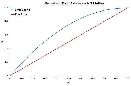
This clearly demonstrates that the nearest neighbor rule's maximum error rate is less than twice of Bayes decision error ($ P \leq 2P^* $). Obviously we can get better error bound by observing the variance where

Applying this equation with previous equation, we will get the desired error bounds on the nearest neighbor rule for infinite number of samples. Figure 2 illustrates the graphical error bound of the nearest neighbor rule.

Metrics Type

However, the closest distance between x' and x is determined by which metrics are used for feature space. A "metric" on a space S is a function $ D: S\times S\rightarrow \mathbb{R} $ which has following 4 properties:

• Non-negativity : $ D(\vec{x_{1}},\vec{x_{2}}) \geq 0, \forall \vec{x_{1}},\vec{x_{2}} \in S $
• Symmetry : $ D(\vec{x_{1}},\vec{x_{2}}) = D(\vec{x_{2}},\vec{x_{1}}), \forall \vec{x_{1}},\vec{x_{2}} \in S $
• Reflexivity : $ D(\vec{x},\vec{x}) = 0, \forall \vec{x} \in S $
• Triangle Inequality : $ D(\vec{x_{1}},\vec{x_{2}}) + D(\vec{x_{2}},\vec{x_{3}}) \geq D(\vec{x_{1}},\vec{x_{3}}), \forall \vec{x_{1}},\vec{x_{2}},\vec{x_{3}} \in S $

Real Application

References

Questions and comments

If you have any questions, comments, etc. please post them on this page.

Back to ECE662, Spring 2014