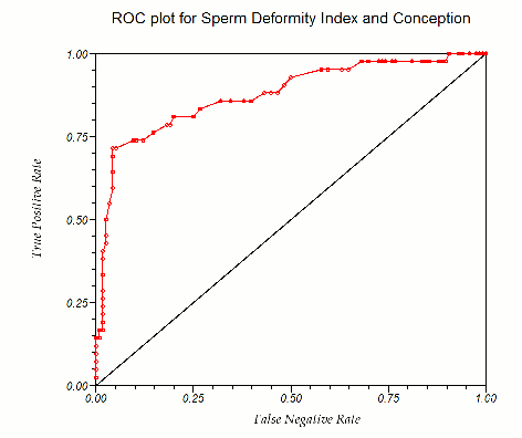
The Receiver Operating Characteristic (ROC) Curve is a commonly-used technique for showing the trade-off between false-positives and false-negatives as a threshold is varied.
Computing the ROC curve
Suppose you have trained a classifier to produce a threshold in the range $ [0 1] $. To produce an ROC curve, you would apply the classifier to your test data, producing a number between 0 and 1 for each sample. Then for each threshold between 0 and 1, you classify the input data and decide if it is correct or not.
Then, for each threshold, you plot the true positive rate against the false positive rate, as illustrated in the following curve.
At the bottom left corner of the curve, we see that a very high threshold will never make a false claim for class 1, but it will never make a true one, either. At the top right, we see that a very low threshold will always choose class 1, so the true positive rate will be 1, but the false positive rate is 1 as well. Fortunately, there are points in the middle where a fairly good true positive rate can be obtained without a very high false-positive rate.
It is possible to compute the curve even more efficiently using cumulative histograms.
Probabilistic Motivation for Varying Thresholds
===================
This is an example of why we may wish to vary the threshold used in a probabilistic sense
In binary classification, a technique will often produce a number ranging from low values when one class is present to high values when the other class is present. We then threshold this number to determine the correct class. For example, consider [Bayes classification]. It is common to look at the log ratio of the two classes:
 .. image:: tex
   :alt: tex: \displaystyle g(x) = log\left(\frac{p(c_1|x)}{p(c_2|x)}\right) = log\ p(c_1|x) - log\ p(c_2|x)
When g(x)>0, class 1 is more likely than class 2, and we select class 1. Applying Bayes' rule, and canceling the p(x):
 .. image:: tex
   :alt: tex:g(x) = log(p(c_1|x)p(c_1)) - log(p(c_2|x)p(c_2))
 .. image:: tex
   :alt: tex:    = [ log\ p(c_1|x) - log\ p(c_2|x) ]  -  [log\ p(c_1) - log\ p(c_2)]
.. |tex1| image:: tex
:alt: tex: p(c_1) = p(c_2)
We often will assume that the clases are equally likely ( |tex1| ) and ignore the second term in the equation above. The ROC curve allows us to generalize this to when the prior probabilities are not known. We lump the ratio of the priors into a threshold, and rename the first half of the equation to g_2, so
 .. image:: tex
   :alt: tex: g(x)  = g_2(x) - T
where
 .. image:: tex
   :alt: tex: T =   [log\ p(c_1) - log\ p(c_2)]
So now class 1 will be chosen if
  .. image:: tex
   :alt: tex: g_2(x) > T
.. |p_1| image:: tex
:alt: tex: p(c_1)
.. |p_2| image:: tex
:alt: tex: p(c_2)
.. |l_p_1| image:: tex
:alt: tex: log\ p(c_1)
.. |l_p_2| image:: tex
:alt: tex: log\ p(c_2)
Because T is the the difference between two logarithms, it can take on any real value. Even though the probabilities |p_1| and |p_2| are constrained to be between 1 and 2, either |l_p_1| and |l_p_2| may be arbitrarily negative when |p_1| or |p_2| is close to 0, so the difference between them can be arbitrarily large.
So even in this theoretical framework, it is necessary to vary a threshold during Bayesian analysis. This happens when we do not know the prior probabilities of the two classes.
Medical Application
=
In medicine, it is very likely for priors to be very different, e.g. 0.99999 probability of not having a disease and 0.00001 probability of having it. [To be expanded....]


