Ece438f19bhenmanbonus - Rhea

Formant Analysis Using Wideband Spectographic Representation

By user:BJH (Brandon Henman)

Topic Background

Like most systems in the real world, the human vocal tract can be broken down and modeled as a system that takes real inputs (vibration of vocal cords) and transforms them (via the vocal tract) into real outputs (human speech).

The vocal system itself resonates certain frequencies, called formant frequencies, depending on how a person changes the shape of their vocal tract in order to pronounce certain phonemes, or "building blocks" of sounds.

This makes sense logically, as our brains classify different phonemes and speech to be different ranges of frequencies in order to process speech signals, otherwise all sounds would mean the same thing!

In order for our brains to have universally recognized phonemes, it follows that a phoneme has roughly the same formant frequencies for everyone, e.g. "you" sounds like "yoo" for everyone.

Interestingly enough, this implies that the variations between individual pitch caused by differences in vocal cord size (which affects the frequency of the vocal folds when voicing signals) does NOT affect the resonant frequencies of the vocal tract.

Think of the vocal tract as a garden hose with a variable-spray nozzle. The water pressure/flow is your vocal cords applying an input to your nozzle, or vocal tract. Your nozzle (vocal tract) then selects which spray settings it wants to shape the water flow into before it spreads out from the end of the hose, which is seen the same by both yourself and the outside world: the same as your speech!

Keeping these concepts in mind, we will use a spectogram-based approach to identify formant frequencies in my speech and compare them to known formant frequencies to both demonstrate how to identify formant frequencies, and to show that formant frequencies are universal.

Audio Files

Here are some examples of voiced phonemes that will be analyzed for their formant frequencies:

-Custom-recorded, 16kHz sampling rate

Me saying "a" :Media:Vowels_voiced_a.wav ("ay")

Me saying "e" :Media:Vowels_voiced_e.wav ("ee")

Me saying "i" :Media:Vowels_voiced_i.wav ("eye")

Me saying "o" :Media:Vowels_voiced_o.wav ("oh")

Me saying "u" :Media:Vowels_voiced_u.wav ("yoo")

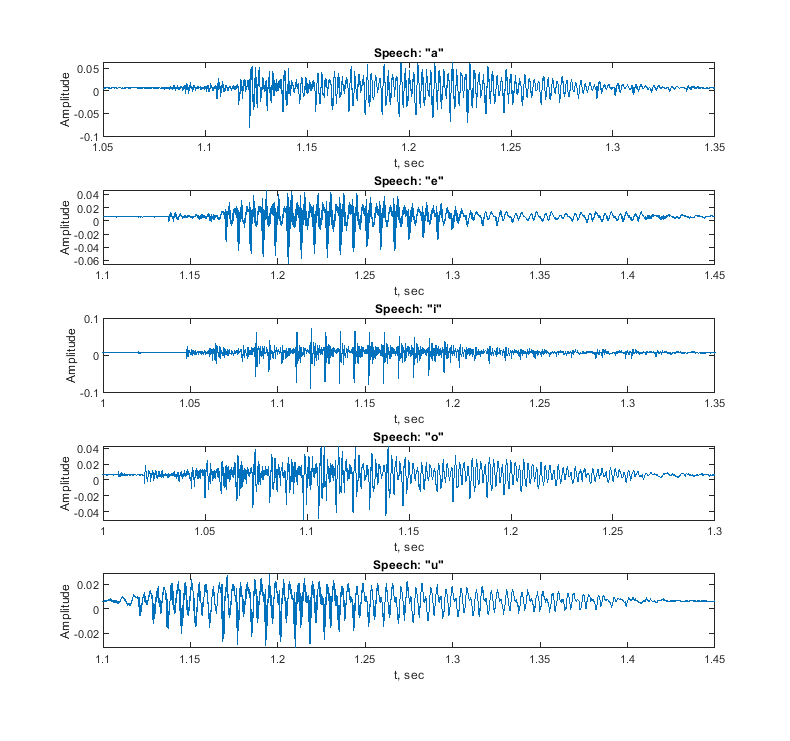
Time Domain Representation of Recorded Signals:

Methodology

Convert the audio to single-channel
Plot time-domain representations of voiced phonemes
Create Spectographic Representations of each signal by applying a shifting N-point DFT window along the length of the input signal and converting the resulting DFT into a column of an output matrix (wideband spectogram)
Identify formant frequencies F1 and F2 at the beginning and end of speech
Compare formant frequencies of custom signals to commonly accepted values of voiced phonemes

Matlab Code

1#- DFT Window Function: This allows us to create the column vectors of our spectogram by performing multiple DFTs across the signal.

   function [X] = DFTwin(x,L,m,N)
   %DFTwin computes the DFT of a windowed length L segment of vector x
   window = hamming(L); %hamming window of desired length L
   x1 = x(m:length(window)+m); %segment of x we want to DFT
   signal = zeros(1,L);
   for z =1:1:length(window)
       signal(z) = x1(z) .* window(z);
   end
   X = fft(signal,N);
   end

2#- Spectogram Function (16kHz compatibility): This allows us to generate our spectogram by piecing together our DFTs using a chosen window length L, overlap value, and value of N for our N-pt dft. Note that These values can be varied to affect the final appearance of the spectogram, but the values below were chosen/tweaked to balance ease of viewing, computation time, and signal detail.

   function [A] = Specgm2(x,L,overlap,N)
   %Specgm creates a spectogram using DFTwin via a matrix of windowed DFTs
   %create a matrix
   for n = 1:1:length(x)
       m = (((n-1) * L) - ((n-1) *overlap)) + 1;
       if ((m+L) > length(x)) %if m + length of window exceeds the signal bounds
           break
       end
       A(:,n) = transpose(DFTwin(x,L,m,N));
   end
   for z = 1:1:(N/2)
       A(1,:) = []; %clear half of the matrix
   end
   A = 20*log10(abs(A)); %convert to dB
   A = flip(A);
   [l,k] = size(A); %#columns and rows in matrix A
   y1 = 0:(1/(length(l))):8000 - (1/(length(k))); %0 to 8kHz
   x1 = 0:(1/16000):length(x)/16000; %16kHz sampling rate
   imagesc(x1,y1,A); %define x and y time/freq. vectors to plot
   colormap(jet)
   axis xy
   end

3#- Main Project Script:

   %{
       ECE438 Bonus Project - Brandon Henman
       Date: 11/15/2019
       Note: Code takes a while to run on slower computers due to the sampling
       rate & the multiple signals being processed. 
   %}

   format rat %fractions are better than decimals
   clear %clear vars
   close all %refresh all figures
   %Load Audio Signals, 16kHz Sampling Rate
   audio_a = transpose(audioread('vowels_voiced_a.wav'));
   audio_e = transpose(audioread('vowels_voiced_e.wav'));
   audio_i = transpose(audioread('vowels_voiced_i.wav'));
   audio_o = transpose(audioread('vowels_voiced_o.wav'));
   audio_u = transpose(audioread('vowels_voiced_u.wav'));
   %convert to single-channel audio (2-channel)
   audio_a = audio_a(1,:);
   audio_e = audio_e(1,:);
   audio_i = audio_i(1,:);
   audio_o = audio_o(1,:);
   audio_u = audio_u(1,:);
   %Play Audio Signals
   %sound(audio_a,16000);
   %sound(audio_e,16000);
   %sound(audio_i,16000);
   %sound(audio_o,16000);
   %sound(audio_u,16000);

   %time plotting vectors
   fs = 16000; %sampling frequency
   N = 1024; %DFT samples
   ta = 1:1:length(audio_a);
   ta = ta./ fs;
   te = 1:1:length(audio_e);
   te = te./ fs;
   ti = 1:1:length(audio_i);
   ti = ti./ fs;
   to = 1:1:length(audio_o);
   to = to./ fs;
   tu = 1:1:length(audio_u);
   tu = tu./ fs;

   %speech signal plots
   figure(1)
   subplot(5,1,1)
   plot(ta,audio_a)
   xlabel('t, sec')
   ylabel('Amplitude')
   title('Speech: "a"')
   xlim([1.05 1.35])
   subplot(5,1,2)
   plot(te,audio_e)
   xlabel('t, sec')
   ylabel('Amplitude')
   title('Speech: "e"')
   xlim([1.1 1.45])
   subplot(5,1,3)
   plot(ti,audio_i)
   xlabel('t, sec')
   ylabel('Amplitude')
   title('Speech: "i"')
   xlim([1 1.35])
   subplot(5,1,4)
   plot(to,audio_o)
   xlabel('t, sec')
   ylabel('Amplitude')
   title('Speech: "o"')
   xlim([1 1.3])
   subplot(5,1,5)
   plot(tu,audio_u)
   xlabel('t, sec')
   ylabel('Amplitude')
   title('Speech: "u"')
   xlim([1.1 1.45])

   %plotting spectograms

   %wideband spec a
   figure(2)
   Specgm2(audio_a,100,80,N);
   xlabel('t')
   ylabel('Hz')
   xlim([1 1.5])
   title('Wideband Spectogram of "a"')

   %wideband spec e
   figure(3)
   Specgm2(audio_e,100,80,N);
   xlabel('t')
   ylabel('Hz')
   xlim([1.07 1.56])
   title('Wideband Spectogram of "e"')

   %wideband spec i
   figure(4)
   Specgm2(audio_i,100,80,N);
   xlabel('t')
   ylabel('Hz')
   xlim([0.98 1.49])
   title('Wideband Spectogram of "i"')

   %wideband spec o
   figure(5)
   Specgm2(audio_o,100,80,N);
   xlabel('t')
   ylabel('Hz')
   xlim([0.99 1.35])
   title('Wideband Spectogram of "o"')

   %wideband spec u
   figure(6)
   Specgm2(audio_u,100,80,N);
   xlabel('t')
   ylabel('Hz')
   xlim([1.05 1.48])
   title('Wideband Spectogram of "u"')

Spectogram Results & Formant Analysis

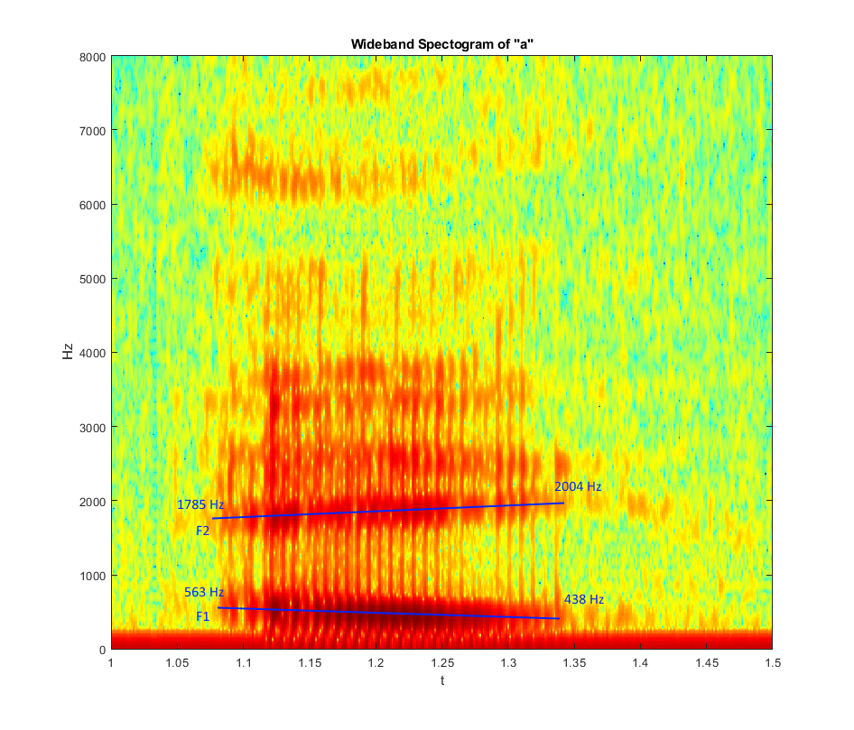
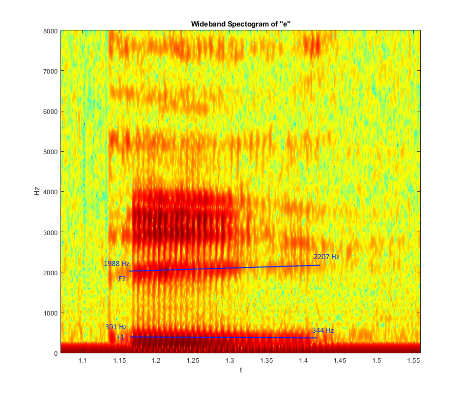
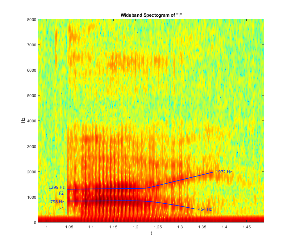
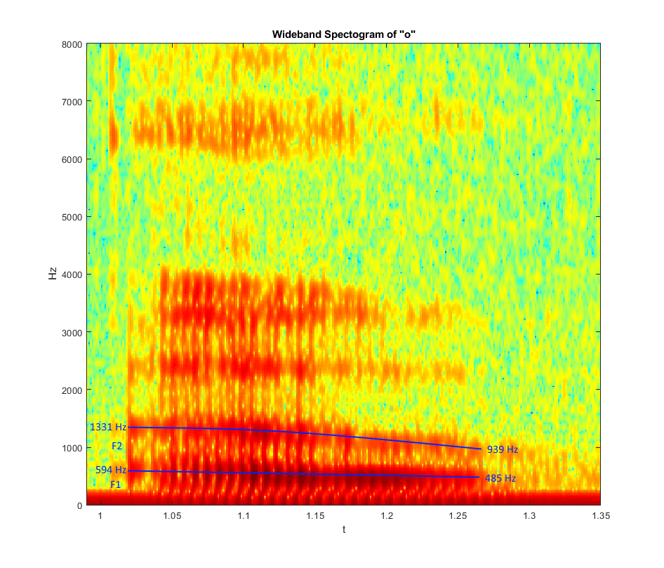
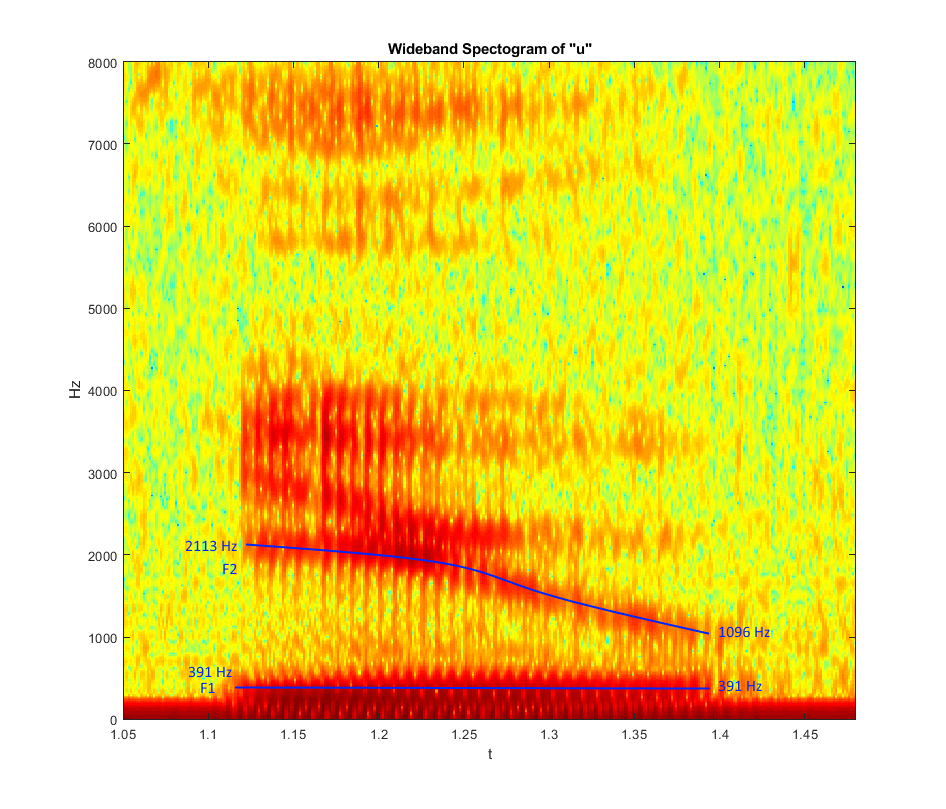
Due to the relatively short window size used to make the wideband spectogram, it is straightforward to identify high-magnitude frequencies across duration of the signal. Additionally, the short window size provides more detail of how the frequency of the signal changes over time, at the cost of less accuracy (a wider formant streak/band) when trying to determine the exact frequency of formants. Here, we approximate formant frequencies to be the approximate center(s) of each formant "streak" on the spectogram, which correspond to resonances in the vocal tract.

Formant frequencies F1 and F2 are the first two streaks (resonances) starting from the bottom of the plot, and are measured near the head and tail ends of each formant "streak" to observe how the formant frequencies shift over the pronunciation of an english vowel.

Note that each spectogram has a streak near the zero-frequency: this is not a speech formant, but rather noise from the input signals and noise due to windowing effects of the spectogram.

Wideband Spectogram of A:

References

- Lecture Notes for ECE438. F19 ed., 2019.
- ECE438 Lab #9: Speech Processing