LAPLACIAN FILTER BLUR DETECTION
INTRODUCTION:
With the advancement of digital photography and development of microelectronics, it has been possible to introduce a larger public to the Digital Camera. More and more people are taking high quality photographs these days and it has been a challenge for companies to enhance the abilities of these cameras. One of the major issues recognized is blurring of an image. The idea of blur correction is to capture the intent of a photographer’s capturing of the image, and make corrections to the actual photograph. A great deal of research has been done on this topic and today, using softwares such as MATLAB and Python, blur detection has become relatively easier and efficient.
A major way to work on blur detection is by extracting certain aspects from the original image automatically and modify these using algorithms. One such way to do so is performing Laplacian on a blurred image. How it works is that this operation detects the rapid changes in intensity in a 2-D image.
STEPS IN EDGE DETECTION: Here are the following steps that are taken for algorithms in edge detection:
1. Filtering: Using gradient computation of Intensity values (in x and y). Both these points are susceptible to noise and hence Gaussian filtering is used to counter this effect. The image is taken in as a set of discrete pixels. Normally, blurring can be achieved on a normal image by passing it through a Gaussian filter, which is a low pass filter and creates ripples, which show up as noise. Hence the Gaussian filter is used to counter this noise, a process called Gaussian smoothing. Laplacian filters being derivative filters, are sensitive to noise and thus this process comes in handy, although it results in decrease of edge strength as noise is cancelled. This is how the equation of a Laplacian filter looks:
Here, I (x,y) is the intensity values, whereas L(x,y) is the laplacian of an image.
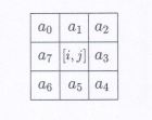
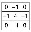
However! There is a little step involved, as mentioned, Gaussian smoothing. To approximate the effects of the Laplacian (above mentioned second derivatives), we include an “approximate discrete convolution kernel”. These kernels look like a 3x3 matrix, in the following form, followed by a commonly used kernel:
Sample Kernel
Commonly used kernel


