Frequency Downsampling - Rhea

Introduction

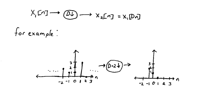
Remember for time domain, Downsampling is defined as:



Now let's describe this process in the frequency domain.

Derivation

First we'll take the Discrete Time Fourier Transform of the original signal and the downsampled version of it.

$ \begin{align} \mathcal{X}_2(\omega) &= \mathcal{F }\left \{ x_2[n] \right \} = \mathcal{F }\left \{ x_1[Dn] \right \}\\ &= \sum_{n=-\infty}^\infty x_1[Dn]e^{-j\omega n} \end{align} $
make the substitution of $ n=\frac{m}{D} $

$ \begin{align} \mathcal{X}_2(\omega) &= \sum_{m=-\infty}^\infty x_1[m]e^{-j\omega \frac{m}{D}} \end{align} $

Downsampled signal will only be nonzero for m equal to multiples of D so:
$ \begin{align} \mathcal{X}_2(\omega) &= \sum_{m=-\infty}^\infty s_d[m]x_1[m]e^{-j\omega \frac{m}{D}} \text{ where}\\ &s_d[m] = \left\{ \begin{array}{ll} 1, & \text{for }m\text{ multiples of } D\\ 0, & \text{else} \end{array} \right.\\ &\text{ or }=\frac{1}{D}\sum_{k=0}^{D-1} e^{jk2\pi \frac{m}{D}} \text{ so:}\\ \mathcal{X}_2(\omega) &= \sum_{m=-\infty}^\infty \frac{1}{D}\sum_{k=0}^{D-1} x_1[m]e^{jk2\pi \frac{m}{D}}e^{-j\omega \frac{m}{D}}\\ &= \frac{1}{D}\sum_{k=0}^{D-1}\sum_{m=-\infty}^\infty x_1[m]e^{-jm\frac{\omega -k2\pi}{D}} \\ \end{align} $

Comparing to
$ \begin{align} \mathcal{X}(\omega) &= \sum_{n=-\infty}^\infty x[n]e^{-jn\omega}\\ \end{align} $

We can rewrite the previous as
$ \begin{align} \mathcal{X}_2(\omega) &= \frac{1}{D}\sum_{k=0}^{D-1} \mathcal{X}(\frac{\omega -2\pi k}{D}) \\ \end{align} $

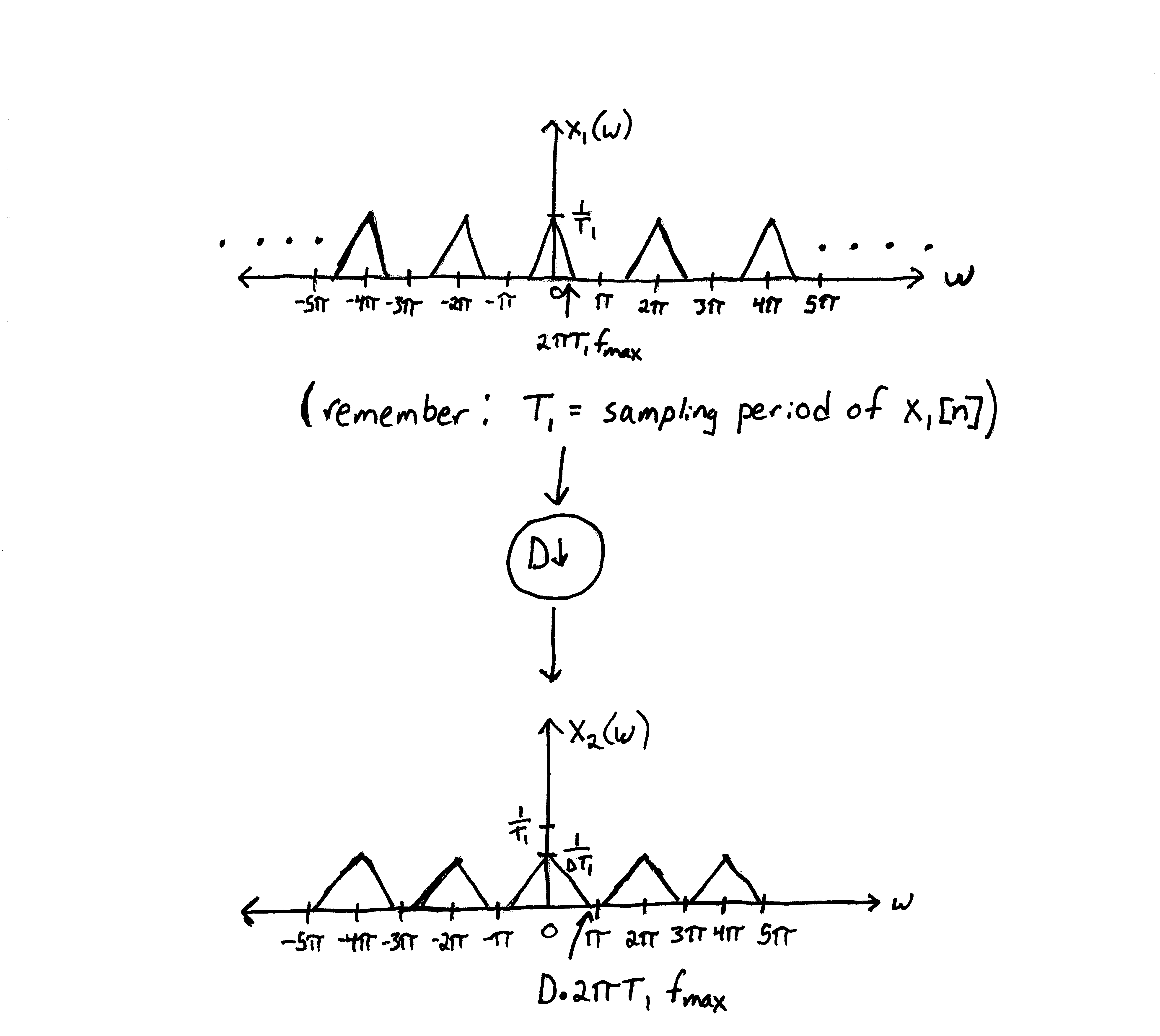
$ \text{Comared to } \mathcal{X}_1(\omega) \text{, } \mathcal{X}_2(\omega) \text{ is } \frac{1}{D} \text{times the magnitude, has its frequencies stretched by }D \text{ and also repeats every }2\pi \text{ (as every DTFT should)} $

Example

It is worth noting that for large enough $ D $ it is possible for the ends of repetitions to overlap, leading to aliasing! To prevent this:

$ \begin{align} D2\pi T_1 f_{max} < \pi\\ \\ x_1[Dn] \text{ has a sampling period of } T_2 = DT_1\text{, so:}\\ \\ \begin{align} \frac{T_2}{T_1}2\pi T_1f_{max} < \pi\\ f_{max} < \frac{1}{2T_2} \end{align} \end{align} $

To make sure this condition is satisfied, we should first pass the original $ x_1[n] $ signal through a low-pass filter with $ f_c = 1/(2T_2) $ BEFORE downsampling.

Since the possible aliasing is caused by the downsampling, trying to low-pass filter after the downsampling will be too late and won't be able to get rid of the aliasing. Thus, the full process of downsampling should look like this:

Image 3

Conclusion

There are two important points to take away about downsampling's effects in the frequency domain:

1. The downsampled signal's frequency spectrum will have its magnitude lowered by the downsampling factor $ D $, and will repeat every $ 2\pi $
2. Downsampling can cause aliasing. To prevent this, we need to lowpass filter BEFORE the downsampling causes any aliasing.