Introduction to Maximum Likelihood Estimation
A slecture by Wen Yi
Partly based on the ECE662 Spring 2014 lecture material of Prof. Mireille Boutin.
Contents
1. Introduction
For density estimation, Maximum Likelihood Estimation (MLE) is a method of parametric density estimation model. When we applying MLE to a data set with fixed density distribution, MLE provides the estimates for the parameters of density distribution model. In real estimation, we search over all the possible sets of parameter values, then find the specific set of parameters with the maximum value of likelihood, which means is the most likely to observe the data set samples.
2. Basic method
Suppose we have a set of n independent and identically destributed observation samples. Then density function is fixed, but unknown to us. We assume that the density funtion belongs to a certain family of distributions, so let θ be a vector of parameters for this distribution family. So, the goal to use MLE is to find the vector of parameters that is as close to the true distribution parameter value as possible.
To use MLE, we first take the joint density function for all the sample observations. For an i.i.d data set of samples, the joint density function is:
As each sample x_i is independent with each other, the likelihood of θ with the data set of samples x_1,x_2,…,x_n can be defined as:
In practice, it’s more convenient to take ln for the both sides, called log-likelihhod. Then the formula becomes: Then, for a fixed set of samples, to maximize the likelihood of θ, we should choose the data that satisfied:To find the maximum of lnL(θ;x_1,x_2,…,x_N ), we take the derivative of θ on it and find theθ value that make the derivation equals to 0.
To check our result we should garentee that the second derivative of θ on lnL(θ;x_1,x_2,…,x_n ) is negative.
3. Practice considerations
3.1 Log-likelihood
As the likelihood comes from the joint density function, it is usually a product of the probability of all the observations, which is very hard to calculate and analyse. Also, as the probability of a observation sample is always less than 1, let's say if one probability for a observation sample is 0.1, then the more data we have, the smaller the likelihood value is (e.g. 0.00000001 or smaller). The small value of likelihood leads to the difficulty in calculating and storing the likelihood.
For the solution of this problem, we took the natural log of the original likelihood, then the joint probability will express as the sum of the natural log of each probability. In this way, the value of likelihood become easier to measure as the number of samples we have increases. Please note that as the probability of one observation of sample is always less than 1, the log-likelihood will always less than 0.
3.2 Removing the constant
Let's take binomial distribution for example, the likelihood for this distribution is:
In this estimation of MLE, we noted that the total number of samples, n, and the number of occurrence, k, is fixed. Then, we can see that as the first part of this likelihood doesn't depend on the value of p, it is a fix value as the value of p changes. So, removing the first part of the likelihood doesn't influence the comparison of likelihood between different value of ps. As a result, we can estimate the likelihood of binomial distribution like following rather than the way above:
3.3 Numerical MLE
Sometimes, we cannot write a equation that can be differentiated to find the MLE parameter estimates, In these cases, we may get exhausted in trying all the value that is possible to be the maximum likelihood. If we choose this method, then the step of the value we try will result in the time of calculation. Thus, we should choose the step as 0.01, 0.001 or 0.0000001 according to the needed accuracy we want.
4. Some basic examples
4.1 Poisson Distribution
For Poisson distribution the expression of probability is:
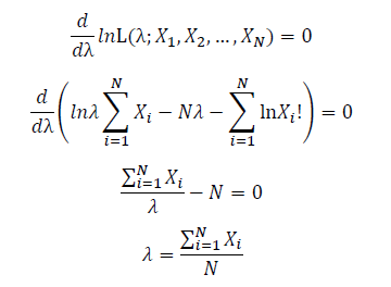
Let X_1,X_2,…,X_N be the Independent and identically distributed (iid) Poisson random variables. Then, we will have a joint frequency function that is the product of marginal frequency functions. The log likelihood of Poisson distribution thus should be:
Take the derivative of λ on it and find theλ value that make the derivation equals to 0.
Thus, the ML estimation for Poisson distribution should be:
4.2 Exponential distribution
For exponential distribution the expression of probability is:
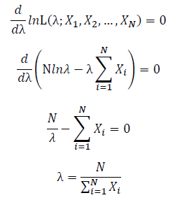
Let X_1,X_2,…,X_N be the Independent and identically distributed (iid) exponential random variables. As P(X=x)=0 when x<0, no samples can sit in x<0 region. Thus, for all X_1,X_2,…,X_N, we can only focus on the x≥0 part. Then, we will have a joint frequency function that is the product of marginal frequency functions. The log likelihood of exponential distribution thus should be:
Take the derivative of λ on it and find theλ value that make the derivation equals to 0.
Thus, the ML estimation for exponential distribution should be:
4.3 Gaussian distribution
For Gaussian distribution the expression of probability is:
Let X_1,X_2,…,X_N be the Independent and identically distributed (iid) Gaussian random variables. Then, we will have a joint frequency function that is the product of marginal frequency functions. The log likelihood of Gaussian distribution thus should be:
Take the derivative of μ,Σ on it and find the μ,Σ value that make the derivation equals to 0.
Thus, the ML estimation for Gaussian distribution should be:
5. Some advanced examples
5.1 Expression of Estimated Parameters
The above estimation all base on the assumption that the distribution to be estimated follows the distribution of a single function, but how about the estimation of the mixture of functions?
To simplify the problem, we only talk about Gaussian Mixture Model (GMM) here. Using the same method, it’s easy to extend it to other kind of mixture model and the mixture between different models.
To start with, we should know that if we set the number of Gaussian function to be used in the GMM estimation flexible, we will find out that the number of Gaussian function will never reach a best solution, as adding more Gaussian functions into the estimation will subsequently improve the accuracy anyway. As calculating how many Gaussian function is include in GMM is a clustering problem. We assume to know the number of Gaussian function in GMM as k here.
As this distribution is a mixture of Gaussian, the expression of probability is:
α_j is the weight of Gaussian function g_j (x).
Following Bayes rule, the responsibility that a mixture component takes for explaining an observation X_i is:
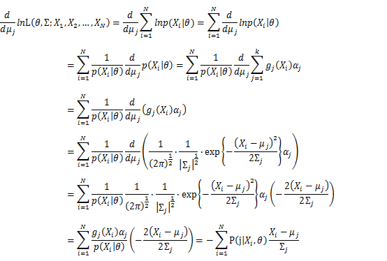
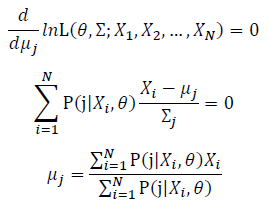
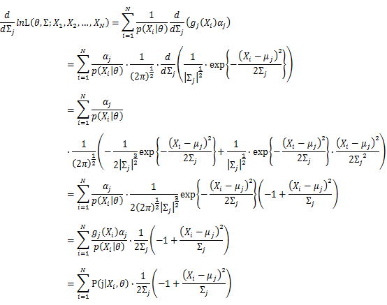
Then, we will have a joint frequency function that is the product of marginal frequency functions. The log likelihood of Gaussian Mixture Model distribution thus should be: Take the derivative of μ_j,Σ_j on it and find the μ_j,Σ_j value that make the derivation equals to 0.The α_j is subject to
Basic optimization theories show that α_j is optimized by:
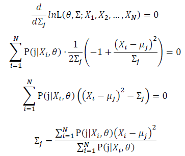
Thus, the ML estimation for Gaussian Mixture Model distribution should be:
5.2 Practical Implementation
Now we can observe that, as the Gaussian Mixture Model with K Gaussian functions have 3K parameters, to find the best vector of parameters set, θ, is to find the optimized parameters in 3K dimension space. As the Gaussian Mixture Model include more Gaussian functions, the complexity of computing the best θ will go incrediblily high. Also, we can see that all the expressions of μ, Σ and α include themselves directly or indirectly, it’s implossible to get the value of the parameters within one time calculation.
Now it’s time to introduce a method for finding maximum likelihood with large number of latent variables (parameters), Expectation–maximization (EM) algorithm.
In statistics, an expectation–maximization (EM) algorithm is an iterative method for finding maximum likelihood estimates of parameters in statistical models, where the model depends on unobserved latent variables (the parameters). The EM iteration alternates between performing an expectation (E) step, which creates a function for the expectation of the log-likelihood evaluated using the current estimate for the parameters, and a maximization (M) step, which computes parameters maximizing the expected log-likelihood found on the E step. These parameter-estimates are then used to determine the distribution of the latent variables in the next E step.
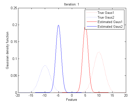
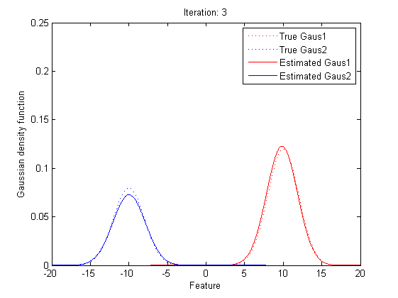
In short words, to get the best θ for our maximum likelihood, firstly, for the expectation step, we should evaluate the weight of each cluster with the current parameters. Then, for the maximization step, we re-estimate parameters using the existing weight.
By repeating these calculation process for several times, the parameters will approach the value for the maximum likelihood.
6. References
www.cscu.cornell.edu/news/statnews/stnews50.pdf
en.wikipedia.org/wiki/Maximum_likelihood
en.wikipedia.org/wiki/Expectation%E2%80%93maximization_algorithm
statgen.iop.kcl.ac.uk/bgim/mle/sslike_1.html
eniac.cs.qc.cuny.edu/andrew/gcml-11/lecture10c.pptx
statweb.stanford.edu/~susan/courses/s200/lectures/lect11.pdf
Statistics and Measurement Concepts with OpenStat, by William Miller]
Questions and comments
If you have any questions, comments, etc. please post them on this page.


