JPEG Compression
Overview
JPEG compression is a lossy compression format for images. Here is a simple explanation of how it works.
Step 1:
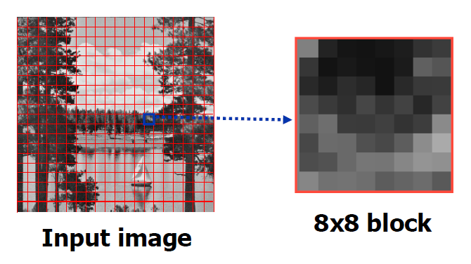
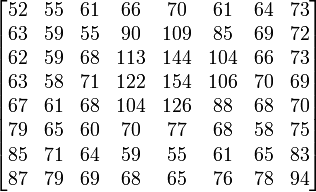
The image is divided into non-overlapping 8 by 8 blocks. If the image width or size does not divide evenly into 8, the image may be cropped or pixels may be added to make the image divisible by 8. Each 8 by 8 block will contain 64 values. For a grayscale image, each pixel may be anywhere from 0 to 255, where 0 is pure black and 255 is pure white.
A sample 8 by 8 block for a grayscale image
Step 2:
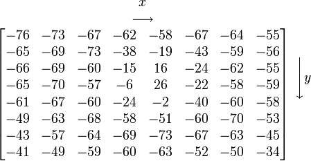
The 2-D Discrete Cosine Transform (DCT) is applied to each 8 by 8 block. For the purposes of applying the DCT, the values in each block are first shifted by -128 to center around zero.
Shift the image by -128 to center pixel values around 0
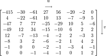
2-D DCT of the zero-centered 8x8 block
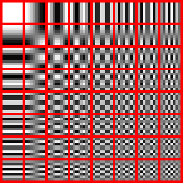
The DCT is chosen over transforms like the FFT because the frequency coefficients are represented by only real numbers. The FFT would require two 8 by 8 matrices, one to store the real part of the frequency coefficient, another to store the imaginary part. The result of the DCT is also an 8 by 8 block, where the top left corner represents the DC or average pixel value for that specific 8 by 8 block. The bottom left corner is an AC coefficient which represents the fastest vertical change. The top right corner is an AC coefficient which represents the fastest horizontal change. The image is represented as a weighted sum of the 64 possible configurations.
Grayscale representation of the AC components of the 2-D DCT
Step 3:
Once the DCT of the 8 by 8 block is obtained, each block is quantized using a quantization matrix. This is where the lossiness of the JPEG format is introduced. Quantization is essentially a divide and floor operation. The quality factor of a JPEG is directly related to quantization matrix.
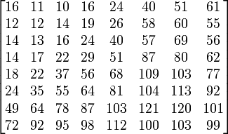
The quantization matrix is an 8 by 8 matrix. Values within this matrix are chosen based on the Q-factor. For an image with high quality, the q-matrix may be set to all 1's. This essentially means no quantization occurs. The way the values in the q-matrix are decided is based upon common trends in an image. Typically, images contain a lot of continuous tones. This makes the DC component of the image and the low AC components particularly dominant in the representation of the image. In a typical image, the majority of the image strength is contained in the top left corner of the 2-D DCT. To preserve these portions of the image, the values in the q-matrix for the top left corner are smaller. The values in the bottom right of the q-matrix are particularly high. This is because the average image is already characterized well with just the top left portion of the 2-D DCT. We don't want to include a high frequency coefficient unless it is particularly dominant and essential to accurate representation. Therefore, the values in the lower right of the q-matrix are high. You can think of this as attenuating high frequency portions of the image unless they have a high signal energy (aka, they're significant in the reconstruction and representation of the image).
Sample quantization matrix
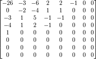
Normally, once you quantize by some value, you would then multiply by the same q value to get the quantized value. So say you had 125 and you wanted to quantize by 16. The quantized value would be 16*floor(125/16). However, this operation is saved for later (by later, I mean decompression of the image). We want to encode what we have now since multiplying by the q-matrix will undoubtedly cause all the numbers to get bigger. When encoding data, smaller values are always better. Below is the quantized DCT without the element-by-element multiplication of the q-matrix.
Quantized DCT coefficients
Step 4:
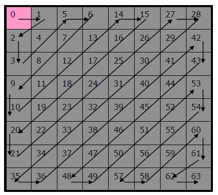
The last step to perform is entropy encoding. The quantized DCT coefficients are arranged in this manner:
How DCT coefficients are ordered prior to encoding
They are ordered this way because the top left of the quantized DCT is where all the values lie. The bottom right will often contain mostly zeroes.
Decompression
When opening a JPEG image, the file is first decoded. The result of the decoded file is the quantized DCT. The first step is multiplying by the quantization matrix used to quantize the image. Then, the Inverse Discrete Cosine Transform (IDCT), is applied. The result is the image, with information loss dependent on the quantization matrix.
Image Sources:
- http://en.wikipedia.org/wiki/JPEG
- Nitin Khana, Purdue University Grad Student

