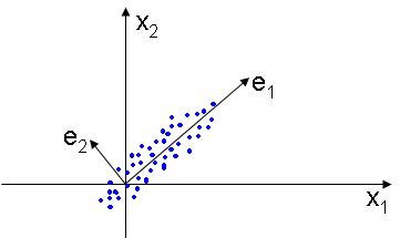
The PCA, or Principal Component Analysis is used to find a lower dimensional subspace that best represents the data, placing the basis of the new linear subspace in the directions that the data varies most. The figure below illustrates this idea:
In order to compute the basis of the new subspace that best represents the data, the PCA diagonalizes the maximum likelihood estimate of the covariance matrix
$ C=\frac{1}{n} \sum_{i=1}^{n} \vec{x_i}\vec{x_i}^T $
by solving the eigenvalue equation
$ C\vec{e} = \lambda \vec{e} $
The solutions to these equations are eigenvalues $ \lambda_1 \lambda_2 \cdots \lambda_m $. Often only $ k m $ eigenvalues will have a nonzero value, meaning that the inherent dimensionality of the data is $ k $, being $ n-k $ dimensions noise in the data.
In order to represent the data in the k dimensional space we first construct the matrix $ E=[\vec{e_1} \vec{e_2} \cdots \vec{e_k}] $. The projection to the new k-dimensional subspace is done by the following linear transformation:
$ \vec{x}^{'} = E^T\vec{x} $
Dimensionality Reduction
By selecting the eigenvectors corresponding to the k largest eigenvalues from the eigenvalue equation, we project the data in a k- dimensional subspace that best represents the data variability in each dimension. In some datasets, many of the eigenvalues $ \lambda_i $ will be zero. This means that the intrinsic dimensionality of the data is smaller than the dimensionality of the input samples.
References
Wikipedia[1]


