(→Part A) |
(→Part A) |
||
| Line 5: | Line 5: | ||
[[Image:sahw1a2_ECE301Fall2008mboutin.jpg]] | [[Image:sahw1a2_ECE301Fall2008mboutin.jpg]] | ||
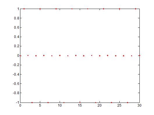
| − | The plot on the left shows the same signal but in DT (y[n] = sin(n)). The sampling frequency is at <math>\pi/2</math> (y[n] = sin(<math>(\pi/2)</math>*n)). The signal repeats itself every 4 sec so that y[n] = y[n+4]. | + | The plot on the left shows the same signal but in DT (y[n] = sin(n)). The sampling frequency is at <math>\pi/2</math> (y[n] = sin(<math>(\pi/2)</math>*n)). The signal repeats itself every 4 sec so that y[n] = y[n+4]. No = k * <math>\frac{2\pi}{\pi/2}</math> ==> No = k * 4 so that the signal repeats itself every 4 seconds. |
[[Image:sahw1a1_ECE301Fall2008mboutin.jpg]] [[Image:sahw1a3_ECE301Fall2008mboutin.jpg]] | [[Image:sahw1a1_ECE301Fall2008mboutin.jpg]] [[Image:sahw1a3_ECE301Fall2008mboutin.jpg]] | ||
Revision as of 17:05, 10 September 2008
Part A
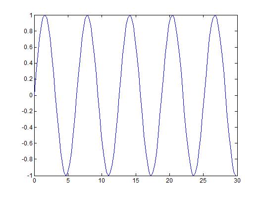
The original signal shown in the first plot is y(t) = sin(t) with a period of $ 2\pi $
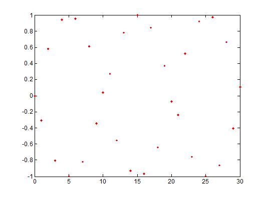
The plot on the left shows the same signal but in DT (y[n] = sin(n)). The sampling frequency is at $ \pi/2 $ (y[n] = sin($ (\pi/2) $*n)). The signal repeats itself every 4 sec so that y[n] = y[n+4]. No = k * $ \frac{2\pi}{\pi/2} $ ==> No = k * 4 so that the signal repeats itself every 4 seconds.


