| Line 67: | Line 67: | ||
<font size = 4> 3. Graphical Example in the Frequency Domain </font> | <font size = 4> 3. Graphical Example in the Frequency Domain </font> | ||
| + | <font size = 3> | ||
| + | <center>[[Image:fig1_deufel.jpeg]]</center> | ||
| + | |||
| + | The first graph shows the signal <math>X_1(w)</math> which is periodic with period 2\pi | ||
| + | |||
| + | The second graph shows the signal <math>X_2(W)</math> which is also periodic with period 2\pi but contains unwanted repetitions of the signal | ||
| + | |||
| + | The third graph shows the Final Signal after it has been passed through the LPF to remove the unwanted repetitions | ||
Revision as of 16:59, 14 October 2014
Upsampling with an emphasis on the frequency domain
By: Michael Deufel
- Introduction
- Derivation
- Examples
- Conclusion
1. Introduction
The purpose of Upsampling is to manipulate a signal in order to artificially increase the sampling rate. This is done by...
- Discretize the signal
- Pad original signal with zeros
- Take the DTFT
- Send through a LPF (low pass filter)
- Take the inverse DTFT to return to the time domain
We will overview the whole process but focus on the effect upsampling has in the frequency domain
2. Derivation
We will start with discrete signal $ x_1[n] $
now we "pad with zeros" to define $ x_2[n] $
$ x_2[n] = \begin{cases}x_1[\frac{n}{D}], & \text{if} \frac{n}{D} \in \mathbb{Z} \\0, &\text{else} \end{cases} f $
note: $ D $ must be an integer greater then one
$ x_2[n] $ can also be defined by
$ x_2[n] = \sum_{k} x_1[k] \delta[n-kD] $
Taking the DTFT of $ x_2[n] $
$ X_2(e^{j\omega}) = \sum_{n} ( \sum_{k} x_1[k] \delta[n-kD]) e^{-j\omega n}) $
switching the order of the summations you can get
$ X_2(e^{j\omega})= \sum_{k}x_1[k] ( \sum_{n}\delta[n-kD]) e^{-j\omega n}) $
where,
$ \sum_{n}\delta[n-kD]) e^{-j\omega n} = e^{-j\omega kD} $
therefor,
$ X_2(e^{j\omega}) = \sum_{k} x_1[k] e^{-j\omega kD} $
This is just the DTFT of the original signal scaled by D
Now LPF with filter that has cutoffs at $ \frac{\pi}{D} $ and $ \frac{- \pi}{D} $ to remove the unwanted repitions
3. Graphical Example in the Frequency Domain

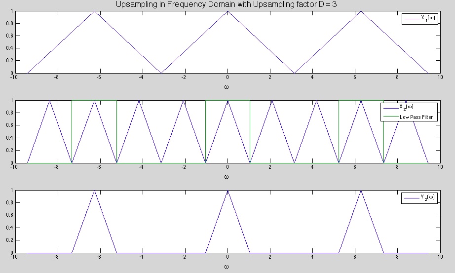
The first graph shows the signal $ X_1(w) $ which is periodic with period 2\pi
The second graph shows the signal $ X_2(W) $ which is also periodic with period 2\pi but contains unwanted repetitions of the signal
The third graph shows the Final Signal after it has been passed through the LPF to remove the unwanted repetitions

