(New page: Category:slecture Category:ECE438Fall2014Boutin Category:ECE Category:ECE438 Category:signal processing <center><font size= 4> Nyquist Theorem, with proof and examp...) |
m |
||
| Line 28: | Line 28: | ||
The Nyquist theorem provides a sufficient condition for perfect reconstruction of a signal from its sampling. In this slecture | The Nyquist theorem provides a sufficient condition for perfect reconstruction of a signal from its sampling. In this slecture | ||
I will give a proof of the Nyquist theorem and give an example demonstrating how perfect reconstruction is possible even when violating the Nyquist condition. | I will give a proof of the Nyquist theorem and give an example demonstrating how perfect reconstruction is possible even when violating the Nyquist condition. | ||
| + | |||
---- | ---- | ||
==Proof== | ==Proof== | ||
| + | |||
| + | Let the ideal sampling <math> x_s(t) \text{ of } x(t) </math> be defined as | ||
| + | |||
| + | <math> x_s(t) := x(t)p_{\frac{1}{f_s}}(t) </math>, | ||
| + | |||
| + | where | ||
| + | |||
| + | <math> p_{\frac{1}{f_s}}(t) = \sum_{k = -\infty}^\infty \delta(t-\frac{k}{f_s}) </math>. | ||
Nyquist Theorem: A signal <math> x(t) </math> that has the property <math> X(f) = 0 </math> for <math> |f| \ge f_M </math> | Nyquist Theorem: A signal <math> x(t) </math> that has the property <math> X(f) = 0 </math> for <math> |f| \ge f_M </math> | ||
can be perfectly reconstructed from its sampling <math> x_s(t) </math> if sampled at a rate <math> f_s > 2f_M </math>. | can be perfectly reconstructed from its sampling <math> x_s(t) </math> if sampled at a rate <math> f_s > 2f_M </math>. | ||
| − | |||
| − | |||
| − | |||
To prove that perfect reconstruction is possible, we must find an expression for <math> x(t) </math> in terms of <math> x_s(t) </math>. | To prove that perfect reconstruction is possible, we must find an expression for <math> x(t) </math> in terms of <math> x_s(t) </math>. | ||
| Line 53: | Line 59: | ||
</math> | </math> | ||
</div> | </div> | ||
| − | |||
| − | + | Without loss of generality, we can assume that the signal <math> x(t) </math> has the spectrum shown in the figure below. The shape of the graph of <math> X(f) </math> does not matter because the only important feature of <math> X(f) </math> is that <math> X(f) = 0 </math> for <math> |f| \ge f_M </math>. | |
[[Image:X1.png]] | [[Image:X1.png]] | ||
| Line 65: | Line 70: | ||
<math> f_s > 2f_M \iff f_s - f_M > f_M \iff -f_s + f_M < f_M </math>. | <math> f_s > 2f_M \iff f_s - f_M > f_M \iff -f_s + f_M < f_M </math>. | ||
| − | + | Together, these inequalities, the graph of <math> X(f) </math>, and the expression for <math> X_s(f) </math> in terms of <math> X(f) </math> imply that <math> X_s(f) </math> will have the spectrum shown in the figure below. | |
[[Image:Xs1.png]] | [[Image:Xs1.png]] | ||
| − | Notice that the spectrum of the ideal sampling of a signal is an amplitude scaled periodic repetition of the original spectrum. Since <math> x(t) </math> is bandlimited and we have sampled at a rate | + | Notice that the spectrum of the ideal sampling of a signal is an amplitude scaled periodic repetition of the original spectrum. Since <math> x(t) </math> is bandlimited and we have sampled at a rate <math> f_s > 2f_M </math>, the periodic repetitions of <math> X(f) </math> do not overlap. |
| − | + | All the information needed to reconstruct <math> X(f) </math> can be found in the portion of <math> X_s(f) </math> that corresponds to <math> X(f) </math> (shown in red). Therefore we can use a simple lowpass filter with gain <math> \tfrac{1}{f_s} </math> and cutoff frequency <math> \tfrac{f_s}{2} </math> to recover <math> X(f) </math> from <math> X_s(f) </math>. | |
| Line 82: | Line 87: | ||
\right. </math> | \right. </math> | ||
| − | <math> \iff x(t) = x_s(t)*sinc(f_st) </math> | + | <math> \iff x(t) = x_s(t)*\text{sinc}(f_st) </math> |
<math> \therefore </math> We can perfectly reconstruct <math> x(t) </math> from <math> x_s(t) </math>. | <math> \therefore </math> We can perfectly reconstruct <math> x(t) </math> from <math> x_s(t) </math>. | ||
| Line 90: | Line 95: | ||
==Example== | ==Example== | ||
| − | Though the Nyquist theorem states that perfect reconstruction is possible if | + | Though the Nyquist theorem states that perfect reconstruction is possible if we satisfy the Nyquist condition <math> (f_s > 2f_M) </math>, it is important to note that this condition is not necessary. The following example demonstrates how perfect reconstruction is sometimes possible even when undersampling. |
Let the signal <math> x(t) </math> have a spectrum <math> X(f) </math> as seen in the figure below. | Let the signal <math> x(t) </math> have a spectrum <math> X(f) </math> as seen in the figure below. | ||
| Line 98: | Line 103: | ||
The Nyquist condition states that we should sample at a rate <math> f_s > 2(2a) = 4a </math>. Instead, let us sample at <math> f_s = 2a </math>. | The Nyquist condition states that we should sample at a rate <math> f_s > 2(2a) = 4a </math>. Instead, let us sample at <math> f_s = 2a </math>. | ||
| − | As before, we have <math> x_s(t) = x(t)p_{\frac{1}{f_s}}(t) | + | As before, we have <math> x_s(t) = x(t)p_{\frac{1}{f_s}}(t) </math> and <math> X_s(f) = f_s\sum_{k = -\infty}^\infty X(f-kf_s) </math> |
<math> \implies X_s(f) = 2a\sum_{k = -\infty}^\infty X(f-2ka) </math>. | <math> \implies X_s(f) = 2a\sum_{k = -\infty}^\infty X(f-2ka) </math>. | ||
| Line 106: | Line 111: | ||
[[Image:Xs2.png]] | [[Image:Xs2.png]] | ||
| − | Notice that | + | Notice that there is no aliasing in <math> X_s(f) </math> even though <math> f_s < 4a </math>. In addition, the portion of <math> X_s(f) </math> that corresponds to <math> X(f) </math> (shown in red) can be recovered using a bandpass filter with gain <math> \tfrac{1}{2a} </math> and cutoff frequencies <math> a \text{ and } 2a </math>. |
---- | ---- | ||
| Line 112: | Line 117: | ||
==Conclusion== | ==Conclusion== | ||
| − | To summarize, the Nyquist theorem states that any bandlimited signal can be perfectly | + | To summarize, the Nyquist theorem states that any bandlimited signal can be perfectly reconstructed from its sampling if sampled at a rate greater than twice its bandwidth <math> (f_s > 2f_M) </math>. However, the Nyquist condition is not necessary for perfect reconstruction as shown in the example above. |
<font size> | <font size> | ||
| Line 119: | Line 124: | ||
---- | ---- | ||
---- | ---- | ||
| − | + | ||
==[[slecture_title_of_slecture_ECE438_review|Questions and comments]]== | ==[[slecture_title_of_slecture_ECE438_review|Questions and comments]]== | ||
Revision as of 06:52, 6 October 2014
Nyquist Theorem, with proof and example
A slecture by ECE student Miguel Rodrigo Castellanos
Partly based on the ECE438 Fall 2014 lecture material of Prof. Mireille Boutin.
Outline
- Introduction
- Proof
- Example
- Conclusion
Introduction
The Nyquist theorem provides a sufficient condition for perfect reconstruction of a signal from its sampling. In this slecture I will give a proof of the Nyquist theorem and give an example demonstrating how perfect reconstruction is possible even when violating the Nyquist condition.
Proof
Let the ideal sampling $ x_s(t) \text{ of } x(t) $ be defined as
$ x_s(t) := x(t)p_{\frac{1}{f_s}}(t) $,
where
$ p_{\frac{1}{f_s}}(t) = \sum_{k = -\infty}^\infty \delta(t-\frac{k}{f_s}) $.
Nyquist Theorem: A signal $ x(t) $ that has the property $ X(f) = 0 $ for $ |f| \ge f_M $ can be perfectly reconstructed from its sampling $ x_s(t) $ if sampled at a rate $ f_s > 2f_M $.
To prove that perfect reconstruction is possible, we must find an expression for $ x(t) $ in terms of $ x_s(t) $.
Given that $ \mathcal{F}(x(t)) = X(f) $, we can find $ X_s(f) $ using the convolution property.
$ \begin{align} X_s(f) &= X(f)*\mathcal{F}(p_{\frac{1}{f_s}})\\ &= X(f)*\mathcal{F}(\sum_{k = -\infty}^\infty \delta(t-\frac{k}{f_s}))\\ &= X(f)*f_s\sum_{k = -\infty}^\infty \delta(f-kf_s)\\ &= f_s\sum_{k = -\infty}^\infty X(f)*\delta(t-\frac{k}{f_s})\\ &= f_s\sum_{k = -\infty}^\infty X(f-kf_s)\\ \end{align} $
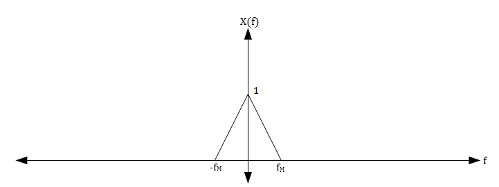
Without loss of generality, we can assume that the signal $ x(t) $ has the spectrum shown in the figure below. The shape of the graph of $ X(f) $ does not matter because the only important feature of $ X(f) $ is that $ X(f) = 0 $ for $ |f| \ge f_M $.
We would like to determine what $ X_s(f) $ looks like in order to find a way to reconstruct $ x(t) $.
Since we have sampled at a rate $ f_s > 2f_M $, the following inequalities hold:
$ f_s > 2f_M \iff f_s - f_M > f_M \iff -f_s + f_M < f_M $.
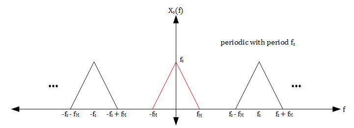
Together, these inequalities, the graph of $ X(f) $, and the expression for $ X_s(f) $ in terms of $ X(f) $ imply that $ X_s(f) $ will have the spectrum shown in the figure below.
Notice that the spectrum of the ideal sampling of a signal is an amplitude scaled periodic repetition of the original spectrum. Since $ x(t) $ is bandlimited and we have sampled at a rate $ f_s > 2f_M $, the periodic repetitions of $ X(f) $ do not overlap.
All the information needed to reconstruct $ X(f) $ can be found in the portion of $ X_s(f) $ that corresponds to $ X(f) $ (shown in red). Therefore we can use a simple lowpass filter with gain $ \tfrac{1}{f_s} $ and cutoff frequency $ \tfrac{f_s}{2} $ to recover $ X(f) $ from $ X_s(f) $.
$ X(f) = X_s(f)\left\{ \begin{array}{ll} \frac{1}{f_s}, & |f| \le \frac{f_s}{2}\\ 0, & \text{else} \end{array} \right. $
$ \iff x(t) = x_s(t)*\text{sinc}(f_st) $
$ \therefore $ We can perfectly reconstruct $ x(t) $ from $ x_s(t) $.
Example
Though the Nyquist theorem states that perfect reconstruction is possible if we satisfy the Nyquist condition $ (f_s > 2f_M) $, it is important to note that this condition is not necessary. The following example demonstrates how perfect reconstruction is sometimes possible even when undersampling.
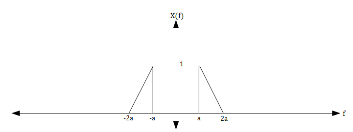
Let the signal $ x(t) $ have a spectrum $ X(f) $ as seen in the figure below.
The Nyquist condition states that we should sample at a rate $ f_s > 2(2a) = 4a $. Instead, let us sample at $ f_s = 2a $.
As before, we have $ x_s(t) = x(t)p_{\frac{1}{f_s}}(t) $ and $ X_s(f) = f_s\sum_{k = -\infty}^\infty X(f-kf_s) $
$ \implies X_s(f) = 2a\sum_{k = -\infty}^\infty X(f-2ka) $.
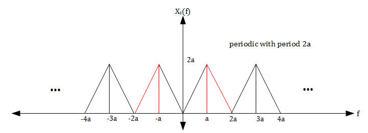
Therefore, $ X_s(f) $ will have the spectrum shown in the figure below.
Notice that there is no aliasing in $ X_s(f) $ even though $ f_s < 4a $. In addition, the portion of $ X_s(f) $ that corresponds to $ X(f) $ (shown in red) can be recovered using a bandpass filter with gain $ \tfrac{1}{2a} $ and cutoff frequencies $ a \text{ and } 2a $.
Conclusion
To summarize, the Nyquist theorem states that any bandlimited signal can be perfectly reconstructed from its sampling if sampled at a rate greater than twice its bandwidth $ (f_s > 2f_M) $. However, the Nyquist condition is not necessary for perfect reconstruction as shown in the example above.
Questions and comments
If you have any questions, comments, etc. please post them on this page.

