| Line 94: | Line 94: | ||
The DTFT of a sampled signal is always periodic with <math>2\pi</math>. So even though the DTFT of a signal sampled below Nyquist may initially not fall within <math>[-\pi,\pi]</math>, it can be extrapolated to the window you are interested in. In my derivation, I chose to shift the cosine before the DTFT. Looking at Figure 3, you can see the comparison between a cosine sampled above and below the Nyquist Rate. The cosine sampled below the Nyquist Rate exhibits aliasing. The aliased signal has a decreased magnitude compared to the original. The aliased signal also is at a different frequency. | The DTFT of a sampled signal is always periodic with <math>2\pi</math>. So even though the DTFT of a signal sampled below Nyquist may initially not fall within <math>[-\pi,\pi]</math>, it can be extrapolated to the window you are interested in. In my derivation, I chose to shift the cosine before the DTFT. Looking at Figure 3, you can see the comparison between a cosine sampled above and below the Nyquist Rate. The cosine sampled below the Nyquist Rate exhibits aliasing. The aliased signal has a decreased magnitude compared to the original. The aliased signal also is at a different frequency. | ||
| + | |||
| + | [[Image:BothNyquist.jpg]] | ||
---- | ---- | ||
Revision as of 16:56, 2 October 2014
DTFT of a Cosine Sampled Above and Below the Nyquist Rate
A slecture by ECE student Sahil Sanghani
Partly based on the ECE438 Fall 2014 lecture material of Prof. Mireille Boutin.
Contents
Outline
- Introduction
- Useful Background
- DTFT Example of a Cosine Sampled Above the Nyquist Rate
- DTFT Example of a Cosine Sampled Below the Nyquist Rate
- Conclusion
- References
Introduction
In this Slecture, I will walk you through taking the DTFT of a pure frequency sampled above and below the Nyquist Rate. Then I will compare the differences between them.
Useful Background
Nyquist Condition: $ f_s = 2f_{max} $
DTFT of a Cosine: $ x_d[n] = cos(2\pi nT){\leftrightarrow}X(\omega) = \pi(\delta(\omega-\omega_o) + \delta(\omega+\omega_o)){ ,for\ } \omega \in [-\pi,\pi] $
The DTFT of a sampled signal is periodic with 2π.
DTFT of a Cosine Sampled Above the Nyquist Rate
For our original pure frequency, let’s choose the E below middle C. The E occurs at 330Hzx(t) = cos(2π * 330t)
Now let’s sample this pure cosine at a frequency above the Nyquist Rate. The Nyquist Rate is:
fs = 2 * fmax = 2 * (330Hz) = 660Hz. Let’s sample at 990Hz.
$ \begin{align} \\ x_d[n] & = x(n*\frac{1}{990Hz})\\ & = cos(2\pi n *\frac{330}{990}) = \frac{e^{j2\pi n \frac{330}{990}} + e^{-j2\pi n \frac{330}{990}}}{2}\\ & = cos(\frac{2\pi n}{3}) \end{align} $
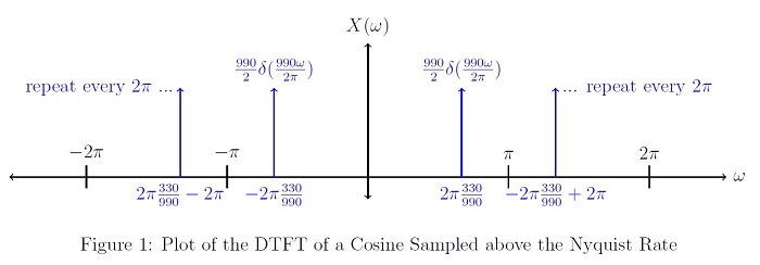
Because $ \left | \frac{2\pi}{3}\right | < \pi $, there is no aliasing occurring in the DTFT, and it can be written as follows:
$ \begin{align} \\ X(\omega) & = \frac{1}{2}(2\pi\delta(\omega - 2\pi \frac{330}{990}) + 2\pi\delta(\omega + 2\pi \frac{330}{990})) , \ \omega \in\ [-\pi,\pi]\\ & = \frac{990}{2}(\delta(\frac{990}{2\pi}\omega - 330) + \delta(\frac{990}{2\pi}\omega + 330)) , \ \omega \in\ [-\pi,\pi]\\ & = rep_{2\pi}(\frac{990}{2}(\delta(\frac{990}{2\pi}\omega - 330) + \delta(\frac{990}{2\pi}\omega + 330))), \forall \omega \end{align} $

DTFT Of a Cosine Sampled Below the Nyquist Rate
Let’s use the same pure frequency as above.x(t) = cos(2π * 330t)
Now let’s sample this pure cosine at a frequency below the Nyquist Rate. From above, the Nyquist Rate is 660Hz. Let’s sample at 550Hz.
$ \begin{align} \\ x_d[n] & = x(n*\frac{1}{550Hz})\\ & = cos(2\pi n *\frac{330}{550}) = \frac{e^{j2\pi n \frac{330}{550}} + e^{-j2\pi n \frac{330}{550}}}{2}\\ \\ \end{align} $
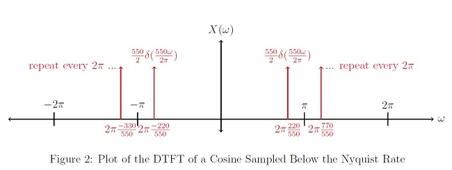
Because $ \pi < \frac{2\pi 330}{550} < 2\pi $, aliasing occurs in the DTFT. The DTFT should be calculated with ω ∈ [ − π, π], so we will use the periodicity of cosine to shift $ x_d[n] $ into an appropriate range.
>$ \begin{align}\\ x_{d}[n] & = cos(2\pi n*\frac{330}{550})\\ & = cos(2\pi n*\frac{330}{550} - 2\pi n)\\ & = cos(2\pi n*(\frac{330}{550} - \frac{550}{550}))\\ & = cos(2\pi n*(\frac{-220}{550}))\\ & = cos(2\pi n*\frac{220Hz}{550Hz}) \end{align} $
Now that the argument of the cosine $ \left | 2\pi \frac{220}{550}\right | < \pi $, we can take the DTFT of xd[n], and the initial value will fall into a desired range for ω.
$ \begin{align} X(\omega) & = \frac{1}{2}(2\pi\delta(\omega - 2\pi \frac{220}{550}) + 2\pi\delta(\omega + 2\pi \frac{220}{550})) , \ \omega \in\ [-\pi,\pi]\\ & = \frac{550}{2}(\delta(\frac{550}{2\pi}\omega - 220) + \delta(\frac{550}{2\pi}\omega + 220)) , \ \omega \in\ [-\pi,\pi]\\ & = rep_{2\pi}(\frac{550}{2}(\delta(\frac{550}{2\pi}\omega - 220) + \delta(\frac{550}{2\pi}\omega + 220))), \forall \omega \end{align} $
Conclusion
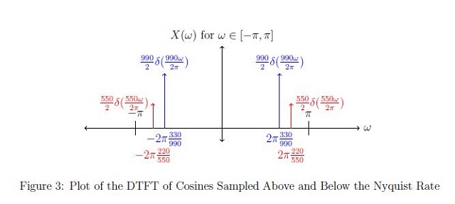
The DTFT of a sampled signal is always periodic with $ 2\pi $. So even though the DTFT of a signal sampled below Nyquist may initially not fall within $ [-\pi,\pi] $, it can be extrapolated to the window you are interested in. In my derivation, I chose to shift the cosine before the DTFT. Looking at Figure 3, you can see the comparison between a cosine sampled above and below the Nyquist Rate. The cosine sampled below the Nyquist Rate exhibits aliasing. The aliased signal has a decreased magnitude compared to the original. The aliased signal also is at a different frequency.
References
[1] Mireille Boutin, "ECE 438 Digital Signal Processing with Applications," Purdue University. September 9, 2014.


