| Line 17: | Line 17: | ||
==[[ECE 301 Fall 2007 mboutin Nyquist Example|Nyquist Example]]== | ==[[ECE 301 Fall 2007 mboutin Nyquist Example|Nyquist Example]]== | ||
{{:ECE 301 Fall 2007 mboutin Nyquist Example}} | {{:ECE 301 Fall 2007 mboutin Nyquist Example}} | ||
| + | |||
| + | ==[[ECE 301 Fall 2007 mboutin Animated Aliasing Example|Animated Aliasing Example]]== | ||
| + | {{:ECE 301 Fall 2007 mboutin Animated Aliasing Example}} | ||
Latest revision as of 12:27, 12 December 2008
Contents
[hide]Convolution Example
Example of CT convolution
This is an example of convolution done two ways on a fairly simple general signal.
- $ x(t) = u(t)\ $
- $ h(t) = {e}^{-\alpha t}u(t), \alpha > 0\ $
Now, to convolute them...
- $ y(t) = x(t)*h(t) = \int_{-\infty}^{\infty}x(\tau)h(t-\tau)d\tau $
- $ y(t) = \int_{-\infty}^{\infty}u(\tau){e}^{-\alpha (t-\tau)}u(t-\tau)d\tau $
- $ y(t) = \int_{0}^{t} {e}^{-\alpha (t-\tau)}d\tau = {e}^{-\alpha t} \int_{0}^{t}{e}^{ \alpha \tau}d\tau $
- $ y(t) = {e}^{-\alpha t}\frac{1}{\alpha}({e}^{\alpha t}-1) = \frac{1}{\alpha}(1-{e}^{-\alpha t}) $
- $ y(t) = \frac{1}{\alpha}(1-{e}^{-\alpha t})u(t) $.
Since $ u(\tau)*u(t-\tau) = 0\ $ when t < 0, also when $ \tau > t\ $, you can set the limit accordingly. Keep in mind the following steps (4&5) are for t > 0, else the function is equal to 0.
Now you can replace the condition in steps 4&5 with a u(t).
Now, the other way... (by the commutative property)
- $ y(t) = h(t)*x(t) = \int_{-\infty}^{\infty}h(\tau)x(t-\tau)d\tau $
- $ y(t) = \int_{-\infty}^{\infty}{e}^{-\alpha (\tau)}u(\tau)u(t-\tau)d\tau $
- $ y(t) = \int_{0}^{t} {e}^{-\alpha \tau}d\tau = \frac{1}{\alpha}(1-{e}^{-\alpha t}) $
- $ y(t) = \frac{1}{\alpha}(1-{e}^{-\alpha t})u(t) $
Since $ u(\tau)*u(t-\tau) = 0\ $ when t < 0, also when $ \tau > t\ $, you can set the limit accordingly. Keep in mind the following step (4) is for t > 0, else the function is equal to 0.
Now you can replace the condition in step 4 with a u(t).
End
Name --dennis.m.snell.1, Sun, 30 Sep 2007 22:25:27
Michael, why did you put your name at the end of this page?
Name --michael.a.mitchell.2, Mon, 01 Oct 2007 15:54:00
Wasn't Sure if the authorship issue had been solved yet. (in class it was said that only the last person to make a change to a page would be credited with it's authorship)
Name --dennis.m.snell.1, Mon, 01 Oct 2007 16:51:27
The authorship issue was not an issue. It was mentioned in class, but by a student asking about it. There is a log of every action and every edit on this kiwi that can be reviewed each week. You are safe in leaving out your name. Sometime soon the editing will be reworked; however, and you might add your name to some other special page, but it will just get lost at the bottom of a topic. I removed your name here, but worry not, you are not forgotten.
... --john.w.fawcett.1, Mon, 15 Oct 2007 11:15:56
why is this under "Exams" as it's parent? Wouldn't Chapter 3 be better?
... --john.w.fawcett.1, Mon, 15 Oct 2007 11:18:06
Sorry, meant Chapter 2. I'll go ahead and add a backlink to chapter 2, but leave this one to Exams up for now.
Frequency and Impulse Response Example
Frequency and Impulse Response of a causal LTI system defined by a difference equation
For the discrete time L.T.I. system described by
- $ y[n]-\frac{1}{2}y[n-1]=x[n]+\frac{1}{2}x[n-1] $
Find the frequency response H($ \omega\ $) and the impulse response h[n] of the system.
Frequency Response:
1: Take the Fourier transform of the equation,
- $ Y(\omega)-\frac{1}{2}e^{-j\omega}Y(\omega)=X(\omega)+\frac{1}{2}e^{-j\omega}X(\omega) $
2: Solve for Y($ \omega\ $)/X($ \omega\ $), which is the frequency response H($ \omega\ $),
- $ H(\omega)=\frac{Y(\omega)}{X(\omega)}=\frac{1+\frac{1}{2}e^{-j\omega}}{1-\frac{1}{2}e^{-j\omega}} $
Impulse Response:
1: Expand into two terms using partial fraction expansion (Guide to Partial Fraction Expansion) to facilitate use of inverse Fourier transform,
- $ H(\omega)=\frac{1}{1-\frac{1}{2}e^{-j\omega}}+\frac{1}{2}\frac{e^{-j\omega}}{1-\frac{1}{2}e^{-j\omega}} $
2: Take the inverse Fourier transform of H($ \omega\ $) (Fourier Transform Table),
- $ h[n]={\left(\frac{1}{2} \right)}^{n}u[n]+\frac{1}{2}{\left(\frac{1}{2} \right)}^{n-1}u[n-1] $
3: Simplify if so inclined,
- for n = 0
- $ h[n] = 1\ $
- for n > 0
- $ h[n] = {\left(\frac{1}{2} \right)}^{n-1} $
Difference Equation in Class Example
Issue with LTI system defined by Difference Equation
I do not understand this difference equation, so could someone please explain it...
The Fourier Transform gives one answer, but it seems as though there are really more answers. One in paticular, c=0, appears to give better results for the step response...please see attached for explanation of what I am talking about...
- $ y[n] - y[n-1] = x[n]\ $
- $ \Rightarrow H(\omega) = \frac{1}{1 - e^{-j \omega}} $
From table in book:
- $ \begin{align} u[n] &\overset {\mathfrak{F}}{\longleftrightarrow} \frac{1}{1 - e^{-j \omega}} + \sum_{k=-\infty}^{\infty} \pi \delta (\omega - 2 \pi k) \\ 1 &\overset {\mathfrak{F}}{\longleftrightarrow} 2 \pi \sum_{l=-\infty}^{\infty} \delta (\omega - 2 \pi l) \end{align} $
- $ \Rightarrow H(\omega) = \frac{1}{1 - e^{-j \omega}} + \sum_{k=-\infty}^{\infty} \pi \delta (\omega - 2 \pi k) - \frac{1}{2} \cdot 2 \pi \sum_{l=-\infty}^{\infty} \delta (\omega - 2 \pi l) $
- $ \Rightarrow h[n] = \mathfrak{F}^{-1}(H(\omega)) = u[n] - \frac{1}{2}\ $
Find step response:
- $ \begin{align} y[n] &= x[n] * h[n] = u[n] * h[n] = \sum_{k=-\infty}^{\infty} u[k]h[n-k] \\ &= \sum_{k=-\infty}^{\infty} u[k] \left ( u[n-k] - \frac {1}{2} \right ) = \sum_{k=-\infty}^{\infty} u[k]u[n-k] - \frac{1}{2} \sum_{k=-\infty}^{\infty} u[k] \\ &= \sum_{k=0}^{\infty} u[n-k] - \frac{1}{2} \sum_{k=0}^{\infty} 1 = -\infty \end{align} $
- (this seems unreasonable!)
Note: The original eq. $ y[n] - y[n-1] = x[n]\ $ can be expressed as:
- $ h[n] - h[n-1] = \delta [n]\ $
By observation, $ h[n] = u[n] + c\ $ for any constant c. And further: the step response is divergent for $ c \ne 0\ $.
So, what is c equal to?
once again --mireille.boutin.1, Fri, 26 Oct 2007 14:30:38
- Dividing by zero is not recommended.
Please clarify --ross.a.howard.1, Fri, 26 Oct 2007 18:16:00
- Can you please clarify where I divided by zero? I still do not know what to do with the arbitrary constant that comes up in the solution...
Nyquist Example
Have you ever looked at a .wav file on a CD to see what frequency it was sampled at? If you do, you'll notice that it is sampled at 44.1 kHz. This is a very significant number because most humans have a hearing range of 20Hz to 20kHz, or a band limited range of about 20kHz. According to the Nyquist sampling theorem, if we want to recreate a sampled signal that is band limited to about 20kHz, then we should sample the signal at twice that frequency.
- 20kHz * 2 = 40kHz
Now if we sample at a slightly higher rate for good measure, we arrive at the 44.1kHz sampling rate, the industry standard for .wav files on CD's.
CD's are also 16-bit audio, which means that each sample will be one of 2^16 or 65,536 different amplitude levels available.
Animated Aliasing Example
Animated Aliasing Example
ECE301 student project
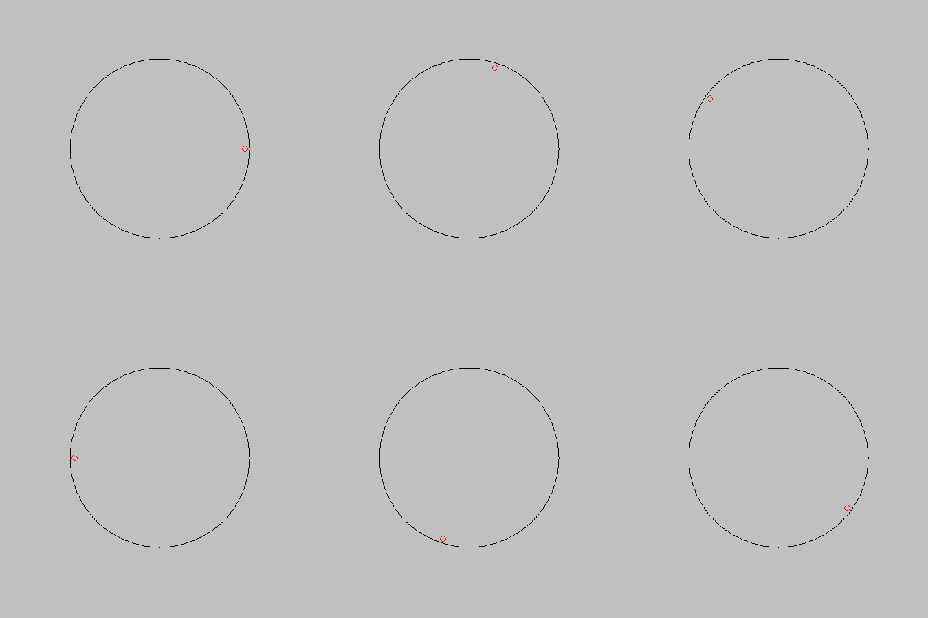
As shown in the Sampling Theorem entry, a signal must be sampled greater than the Nyquist Rate in order to reconstruct the original signal. The effect of undersampling, or sampling at a rate below that of the Nyquist Rate, is aliasing. The example used in class was that of a spinning wheel.
Below is an animation that shows the spinning wheel example in greater detail. The wheel is spinning in the clockwise direction at a rate of 5 sec/rev which corresponds to a frequency of .2 rev/sec. This frequency is the frequency of the signal. The small red dot is just an indicator on a part of the wheel to make it easy to see how the wheel is spinning. In each of the following three cases, the wheel is observed at snap shots in time by using a strobe light. Each case has a different strobe light frequency. This frequency is our sampling frequency.
Case 1: Sampling Frequency (Strobe Light Frequency) = 2 samples/sec (Strobe Flashes Once every .5 Seconds)
- Since the sampling frequency is greater than the Nyquist Rate (The frequency is actually 10 times that of the spinning frequency), then our signal should be able to be reconstructed.
Case 2: Sampling Frequency (Strobe Light Frequency) = .2 samples/sec (Strobe Flashes Once every 5 Seconds)
- Since the sampling frequency is the same as the spinning wheel frequency, (less than the Nyquist Rate) we can expect the motion of the wheel to not be reconstructed properly. Since the sampling frequency is the same as the frequency of the spinning wheel, the wheel appears to be motionless, even though it is still spinning at .2 rev/sec.
Case 3: Sampling Frequency (Strobe Light Frequency) = 2/9 samples/sec (Strobe Flashes Once every 4.5 Seconds)
- In this case, the sampling frequency is higher than that of the frequency of the spinning wheel, but it is again below the Nyquist Rate, so we can expect the motion of the wheel to not be reconstructed properly. Since the sampling frequency is slightly greater than the wheel's frequency, the wheel appears to be spinning backwards.
Note: Watch Carefully, the dot moves very slowly
Discussion
Look! This page is now referenced and reviewed on Stumbleupon! See here


