| Line 53: | Line 53: | ||
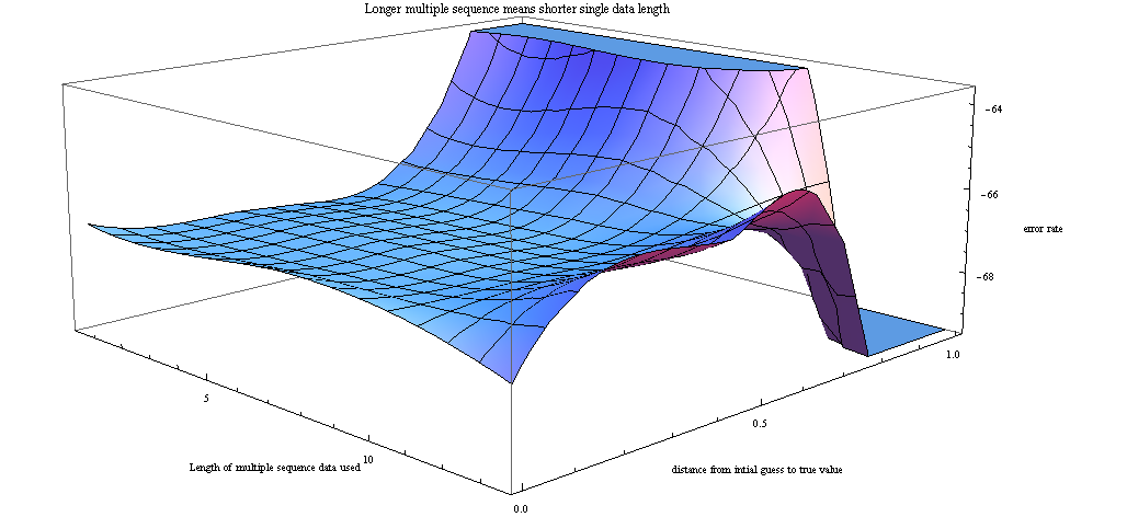
This figure shows the different likelihood of the learned HMM model, vs the different settings of training data used. One can see that the result conforms with the previous figure: where the error rate is larger, the likelihood tends to be lower. | This figure shows the different likelihood of the learned HMM model, vs the different settings of training data used. One can see that the result conforms with the previous figure: where the error rate is larger, the likelihood tends to be lower. | ||
[[Image:EE662Sp10_HMM_lik.png]] | [[Image:EE662Sp10_HMM_lik.png]] | ||
| + | |||
| + | --[[User:Yuanl|Yuanl]] 11:03, 29 April 2010 (UTC) | ||
| + | |||
| + | ---- | ||
| + | [[2010_Spring_ECE_662_mboutin|back to ECE662, Spring 2010, Prof. Boutin]] | ||
Revision as of 06:03, 29 April 2010
Introduction to Hidden Markov Model
Introduction
Hidden Markov Model (HMM) can be categorized into the greater genre of "Probabilistic Graphical Models" -> "Markov Networks" -> 1D Markov Chain of a Mixture Model, (where each chain node contains a hidden state and corresponding emission probabilities). Because of the specialty of Hidden Markov Models, lots of specific algorithms are developed.
Given the following definition of a Hidden Markov Model, define Hidden Markov Model as $ \left\{\mathcal{Z}, \mathcal{X}, A, \pi, \phi \right\} $, where $ \mathcal{Z}=\left\{z_1 \cdots z_T | \forall i, z_i \in \mathcal S:{s_1 \cdots s_K}\right\} $ is a sequence of random variable z which represent the underlying (hidden) states. $ \mathcal{X}=\left\{x_1 \cdots x_T | \forall i, x_i \sim \phi(x|z)\right\} $ is a sequence of observations from a random variable $ x_i $ which is conditioned on the corresponding state $ z_i $.
The following 3 problems are the major research problems for HMM: 1. Evaluation problem: Given a model specification, how to calculate the probability of this model, generating a specific sequence of observations of X.
2. Decoding problem: Given an observation sequence X, how to calculate the most probable state transition sequence Z on a give HMM.
3. Learning problem: Given the training data, observation sequence(s) X, and basic model structure, (i.e. number of states, number of possible observations) how to learn the distributions $ \phi $, $ \pi $ and transition matrix $ A $.
In order to solve these problems, the following algorithms are proposed:
1. The forward algorithm: This algorithm is used to solve the evaluation problem. It takes the HMM model definition, and calculates the probability of an observation sequence X iteratively from $ X_1 $ to $ X_n $.
2. The backward algorithm: This algorithm computes the probability of the $ Z_i $ variable being in a hidden state $ s_i $. iteratively backwards from the nth step, where the probability is calculated by the forward algorithm.
3. The Baum Welch algorithm: In order to learn an HMM model from given training data, by using forward and backward algorithm, and plugging them into an EM algorithm framework, the Baum Welch algorithm can learn a parameter of HMM model which converges to the nearest local maximum likelihood, given the initial parameter settings.
Observations
I implemented Baum Welch algorithm, and would like to illustrate my observations below: The experiment is carried on synthetic data generated with a specific 2 state, 4 output HMM model.
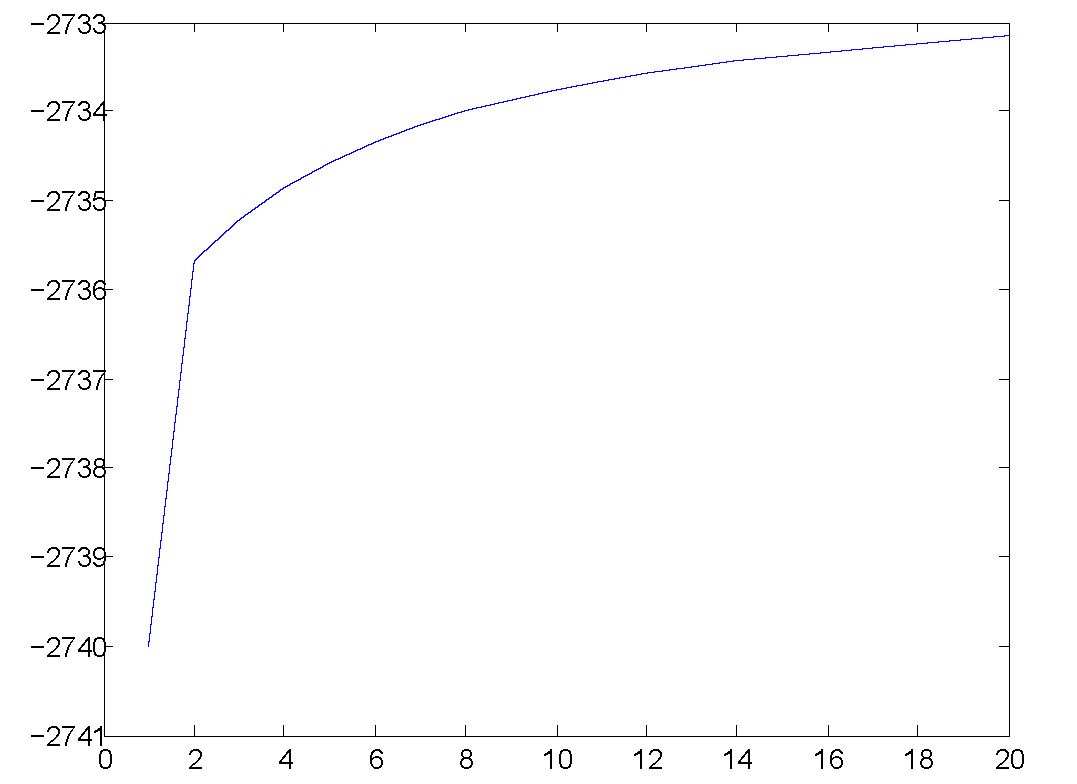
This figure shows the likelihood of the learned model is increasing as the EM algorithm iterates.

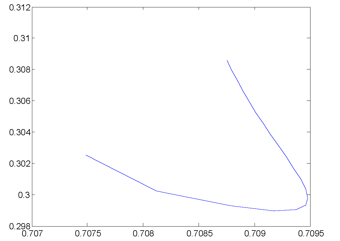
This figure shows the path of the learned transition matrix parameter of changing as the iterations goes on.

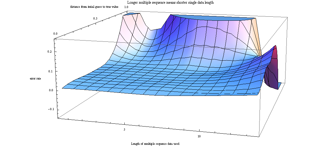
The most interesting observation, however, is that I found training HMM model on many short observation sequences does not compete with training the HMM model on just a few longer observation sequences. The following figures showed that:
This figure shows the different testing error rate of the learned HMM model, with respect to different settings of training data used. The X axis is the number of training data used, if the number is larger, it means I'm using shorter length of each observation sequence. Y axis is the distance of initial guess to the true parameters. The further it is, the worse the result is.

This figure shows the different likelihood of the learned HMM model, vs the different settings of training data used. One can see that the result conforms with the previous figure: where the error rate is larger, the likelihood tends to be lower.

--Yuanl 11:03, 29 April 2010 (UTC)

