| Line 16: | Line 16: | ||
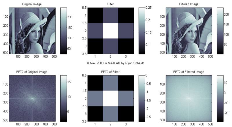
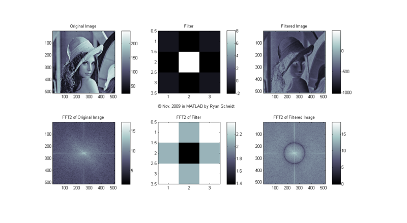
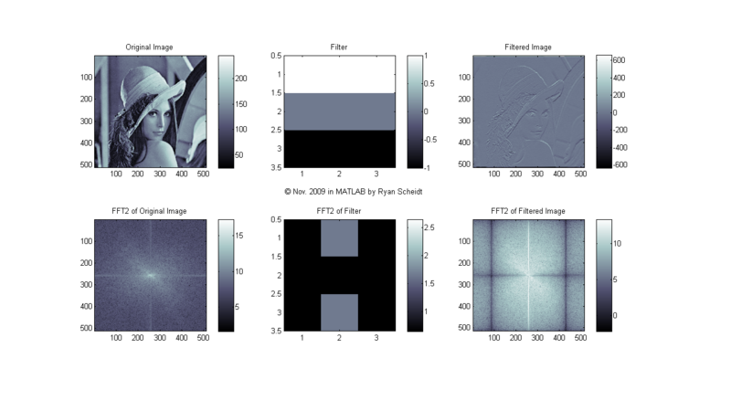
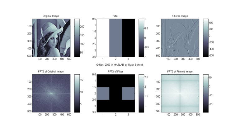
Let's look at what the 2-D FFT of Lena looks like. We will look at some simple 3X3 filters that are then convolved with the original image to create a filtered image. | Let's look at what the 2-D FFT of Lena looks like. We will look at some simple 3X3 filters that are then convolved with the original image to create a filtered image. | ||
| − | The following pictures show the original image (Lena), the image of the filter, and the filtered image (done with conv2). MATLAB m-files available upon request. The colormaps to the right of each image show the corresponding values for each shade of gray (i.e. continuum from white to black). Each image is "normalized to 256 values" so the lowest values (even if negative) are mapped to | + | The following pictures show the original image (Lena), the image of the filter, and the filtered image (done with conv2). MATLAB m-files available upon request. The colormaps to the right of each image show the corresponding values for each shade of gray (i.e. continuum from white to black). Each image is "normalized to 256 values" so the lowest values (even if negative) are mapped to 0 (black) and the highest values are mapped to 255 (white). |
''Note: click on following images and follow "Full resolution" hyperlink to see full image (e.g. 1280 pixels wide).'' | ''Note: click on following images and follow "Full resolution" hyperlink to see full image (e.g. 1280 pixels wide).'' | ||
Revision as of 12:56, 25 November 2009
Spectral Analysis of 2D Signals (December 1, 2009)
Here, I will describe and explain the basics behind analyzing the spectrum of 2-D signals - principally images! - Ryan Scheidt
The following image, commonly referred to as "Lena" (sometimes also "Lenna"), is a famous image utilized in standard image processing algorithms and testing. The background behind this image is quite interesting. Here are some links for the interested reader: [1], [2]
Spectral analysis of two-dimensional signals is not much different than the familiar one-dimensional FFT that we are (more) accustomed to. The only difference is that our signals are now represented in one more plane. We can think of this difference (1D vs. 2D) as the difference between, say, a one-dimensional longitudinal wave in a slinky (like this: [3]), versus a two-dimensional wave from a trampoline (e.g. drop a baseball in the center (or given any other excitation), and the wave will propagate in both x and y-directions ([4]).
Let's look at what the 2-D FFT of Lena looks like. We will look at some simple 3X3 filters that are then convolved with the original image to create a filtered image. The following pictures show the original image (Lena), the image of the filter, and the filtered image (done with conv2). MATLAB m-files available upon request. The colormaps to the right of each image show the corresponding values for each shade of gray (i.e. continuum from white to black). Each image is "normalized to 256 values" so the lowest values (even if negative) are mapped to 0 (black) and the highest values are mapped to 255 (white).
Note: click on following images and follow "Full resolution" hyperlink to see full image (e.g. 1280 pixels wide).


