| Line 24: | Line 24: | ||
"Almost Possible in the Real World" | "Almost Possible in the Real World" | ||
[[Image:Milo.jpg]] | [[Image:Milo.jpg]] | ||
| + | |||
---- | ---- | ||
| Line 79: | Line 80: | ||
[[Image:Milo_original.jpg]] | [[Image:Milo_original.jpg]] | ||
| + | |||
| + | *As we can see, it is an extremely high res-image with clear details | ||
| + | *Now let's down-sample this puppy and see what happens | ||
| + | ---- | ||
| + | [[Image:Milo_downsampled.jpg]] | ||
Revision as of 00:38, 23 September 2009
Contents
Discrete Time Interpolation
Mathematically, sure. Realistically? Let's find out.
Introduction
My fascination with the concept of discrete time interpolation began, when I asked Prof. Boutin if a discrete time interpolator, can ideally make a low-resolution image, a high resolution one.
The answer was, yes. Ideally, it can.
The equations that led to the concept seemed impeccable and mathematically, it seemed to make perfect sense.
But essentially, all we are doing is:
- adding zeros in between samples (the result of which looks horrible by the way)
- Low pass filtering,
and Voila! hi-res image. Impossible right?
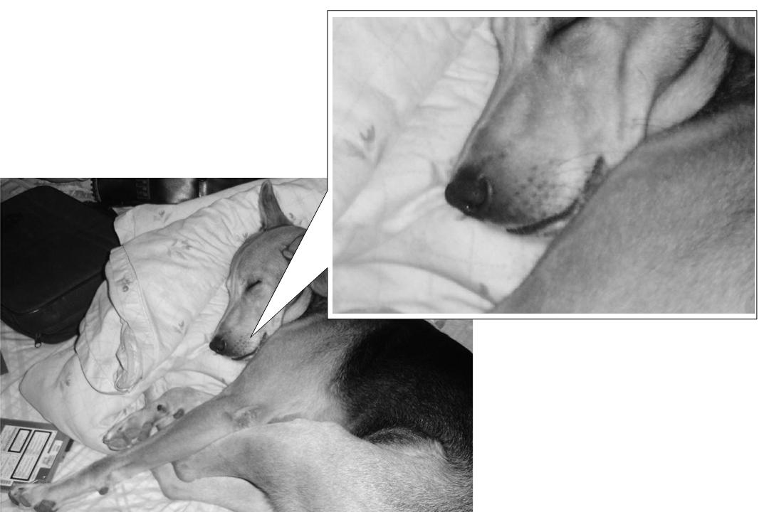
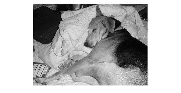
After 6 hours of MATLAB code, and processing the image of my dog "Milo"(shown below), countless times, I am proud to say, that it is
"Almost Possible in the Real World"
Page Map
This page contains
- Application to Actual 1-D signal
- Application to an actual real-world image
Mathematical Basis
To put the math in a nutshell, so that we can get started with the cool stuff,
let's consider the diagrams below:
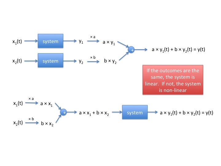
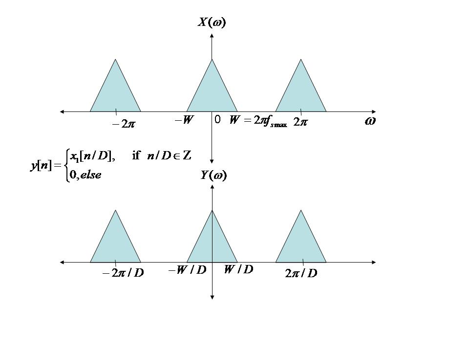
- This shows the basic schematic of an interpolator. D in the circle is how many zeros we fill between samples and the Low Pass Filter removes the extraneous copies of the signal beyond W/D shown in the output below.
- Let's pretend we waved the math wand and got the frequency domain as below.
[Application to Actual 1-D signal]
- Now, let's see if this can be applied to an actual example.
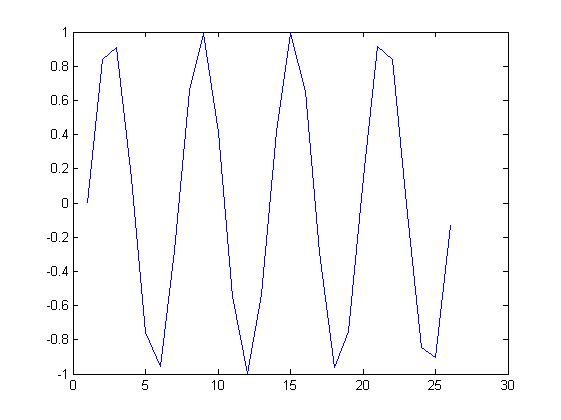
- From the introduction, our main aim was to take a badly sampled signal(our friendly sine wave shown below) and make it "good" or sampled at a better resolution
- According to the math, this whole process should give the same result,as if we were to take a "good" sampling of the original ct signal
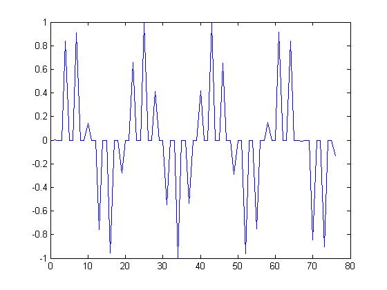
- So, let's see what happens with the insertion of zeros
- Obviously, the signal now contains more samples, as we can see from the x-axis plot.
- Also, the zeros cause the addition of "spikes" in the signal, because now the jumps between samples are higher
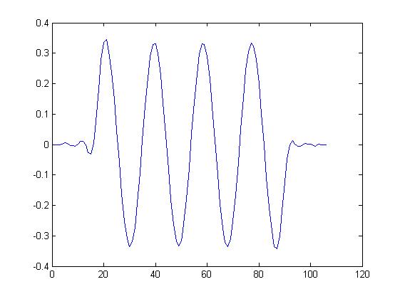
- So, intuitively, we want to use an LPF (low pass filter) to "remove" these high frequency spikes.
- Success!! High-Res Signal
- The low pass filter added a few extraneous samples, for those amongst you who are suspicious as to why we have more samples. I used an FIR Parks Mc Clellen filter in MATLAB, and that usually does this.
Application to Real-World Image
- Now for the coup de grâce: Working with an actual image
- We know we can make 1-D signals work, but images are much more complex
- So the way to test if upsampling works, and indeed makes images better is to have a sloppy image in the first place right?
- Well,that is kinda hard for our megapixel-jaded generation.
- In that case, let's create a low-res image by downsampling a good one
- First, let's see the original
- As we can see, it is an extremely high res-image with clear details
- Now let's down-sample this puppy and see what happens

